Semantic Graph for Text Understanding
In this project, we treat text as a semantic graph rather than a flat sequence of words. From Wikipedia biographies of modern artists, we build a graph where nodes are meaningful word pairs and edges connect them when they appear together or in related contexts. Each node carries a transformer embedding, and a Graph Neural Network learns to “rewire” this graph—strengthening important links, downplaying weak ones, and revealing which artists and concepts truly sit close together or far apart in meaning.
This semantic graph becomes a foundation for NLP tasks: it supports richer recommendations (finding both similar and contrastive artists or documents), cleans and enriches the underlying knowledge graph, and provides structure-aware representations that go beyond simple embedding cosine similarity. Instead of just asking “how similar are these texts?”, we can ask “how is their semantic neighborhood wired?” and let Graph AI answer from the topology of the semantic graph itself.
Conference & Publication
This work was presented at FRUCT35, the 35th Conference of the Open Innovations Association, held in Tampere, Finland, from 24–26 April 2024, as the paper “Enhancing NLP through GNN-Driven Knowledge Graph Rewiring and Document Classification”. It was published in the conference proceedings with the doi: 10.23919/FRUCT61870.2024.10516410 .
GNN Graph Classification for Semantic Graphs
In our previous studies, we focused on the exploration of knowledge graph rewiring to uncover unknown relationships between modern art artists. In one study 'Building Knowledge Graph in Spark Without SPARQL', we utilized artist biographies, known artist relationships, and data on modern art movements to employ graph-specific techniques, revealing hidden patterns within the knowledge graph.In more recent study 'Rewiring Knowledge Graphs by Link Predictions' our approach involved the application of GNN link prediction models. We trained these models on Wikipedia articles, specifically focusing on biographies of modern art artists. By leveraging GNN, we successfully identified previously unknown relationships between artists.
This study aims to extend earlier research by applying GNN graph classification models for document comparison, specifically using Wikipedia articles on modern art artists. Our methodology will involve transforming the text into semantic graphs based on co-located word pairs, then generating subsets of these semantic subgraphs as input data for GNN graph classification models. Finally, we will employ GNN graph classification models for a comparative analysis of the articles.
Introduction
The year 2012 marked a significant breakthrough in the fields of deep learning and knowledge graphs. It was during this year that Convolutional Neural Networks (CNN) gained prominence in image classification with the introduction of AlexNet. At the same time, Google introduced knowledge graphs, which revolutionized data integration and management. This breakthrough highlighted the superiority of CNN techniques over traditional machine learning approaches across various domains. Knowledge graphs enriched data products with intelligent and magical capabilities, transforming the way information is organized, connected, and understood.For several years, deep learning and knowledge graphs progressed in parallel paths. CNN deep learning excelled at processing grid-structured data but faced challenges when dealing with graph-structured data. Graph techniques effectively represented and reasoned about graph structured data but lacked the powerful capabilities of deep learning. In the late 2010s, the emergence of Graph Neural Networks (GNN) bridged this gap and combined the strengths of deep learning and graphs. GNN became a powerful tool for processing graph- structured data through deep learning techniques.
GNN models allow to use deep learning algorithms for graph structured data by modeling entity relationships and capturing structures and dynamics of graphs. GNN models are being used for the following tasks to analyze graph-structured data: node classification, link prediction, and graph classification. Node classification models predict label or category of a node in a graph based on its local and global neighborhood structures. Link prediction models predict whether a link should exist between two nodes based on node attributes and graph topology. Graph classification models classify entire graphs into different categories based on their graph structure and attributes: edges, nodes with features, and labels on graph level.
GNN graph classification models are developed to classify small graphs and in practice they are commonly used in the fields of chemistry and medicine. For example, chemical molecular structures can be represented as graphs, with atoms as nodes, chemical bonds as edges, and graphs labeled by categories.
One of the challenges in GNN graph classification models lies in their sensitivity, where detecting differences between classes is often easier than identifying outliers or incorrectly predicted results. Currently, we are actively engaged in two studies that focus on the application of GNN graph classification models to time series classification tasks: 'GNN Graph Classification for Climate Change Patterns' and 'GNN Graph Classification for EEG Pattern Analysis'.
In this post, we address the challenges of GNN graph classification on semantic graphs for document comparison. We demonstrate effective techniques to harness graph topology and node features in order to enhance document analysis and comparison. Our approach leverages the power of GNN models in handling semantic graph data, contributing to improved document understanding and similarity assessment.
To create semantic graph from documents we will use method that we introduced in our post 'Find Semantic Similarities by GNN Link Predictions'. In that post we demonstrated how to use GNN link prediction models to revire knowledge graphs. For experiments of that study we looked at semantic similarities and dissimilarities between biographies of 20 modern art artists based on corresponding Wikipedia articles. One experiment was based on traditional method implemented on full test of articles and cosine similarities between reembedded nodes. In another scenario, GNN link prediction model ran on top of articles represented as semantic graphs with nodes as pairs of co-located words and edges as pairs of nodes with common words.
In this study, we expand on our previous research by leveraging the same data source and employing similar graph representation techniques. However, we introduce a new approach by constructing separate semantic graphs dedicated to each individual artist. This departure from considering the entire set of articles as a single knowledge graph enables us to focus on the specific relationships and patterns related to each artist. By adopting this approach, we aim to capture more targeted insights into the connections and dynamics within the knowledge graph, allowing for a deeper exploration of the relationships encoded within the biographies of these artists.
Methods
The input data for GNN graph classification models consists of a collection of labeled small graphs composed of edges and nodes with associated features. In this section we will describe data processing and model training in the following order:- Text preprocessing to transform raw data to semantic graphs.
- Node embedding process.
- The process of semantic subgraph extraction.
- Training GNN graph classification model.
From Raw Data to Semantic Graph
To transform text data to semantic graph with nodes as co-located word pairs we will do the following:- Tokenize Wikipedia text and exclude stop words.
- Get nodes as co-located word pairs.
- Get edges between nodes.
- Build semantic graph.
if pair1=[leftWord1, rightWord1],
   pair2=[leftWord2, rightWord2]
   and rightWord1=leftWord2,
then there is edge12={pair1, pair2}
Node Embedding
To translate text of pairs of co-located to vectors we will use transformer model from Hugging Face: 'all-MiniLM-L6-v2'. This is a sentence-transformers model that maps text to a 384 dimensional vector space.
Extract Semantic Subgraphs
As input data for GNN graph classification model we need a set of labeled small graphs. In this study from each document of interest we will extract a set of subgraphs. By extracting relevant subgraphs from both documents, GNN graph classification models can compare the structural relationships and contextual information within the subgraphs to assess their similarity or dissimilarity. One of the ways to extract is getting subgraphs as neighbors and neighbors of neighbors of nodes with high centralities. In this study we will use betweenness centrality metrics.
Train the Model
The GNN graph classification model is designed to process input graph data, including both the edges and node features, and is trained on graph-level labels. In this case, the input data structure consists of the following components:
- Edges in a graph capture the relationships between nodes.
- Nodes with embedded features would be embedded into the nodes to provide additional information to the GNN graph classification model.
- Graph-level labels are assigned to the entire graph, and the GNN graph classification model leverages these labels to identify and predict patterns specific to each label category.
Experiments
Data Source
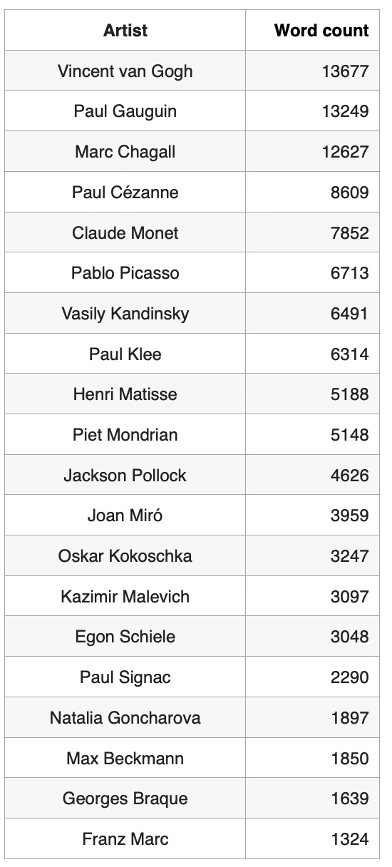
As the data source for this study we used text data from Wikipedia articles about 20 modern art artists. Here is the list of artists and Wikipedia text size distribution: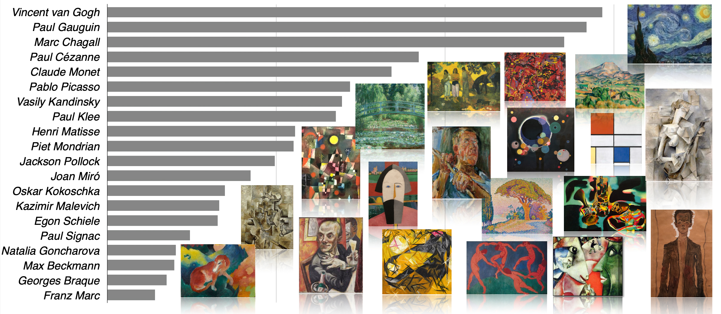
Based on Wikipedia text size distribution, the most well known artist in our artist list is Vincent van Gogh and the most unknown artist is Franz Marc:
 More detail information is available in our post 'Rewiring Knowledge Graphs by Link Predictions'.
To estimate document similarities based on GNN graph classification model, we experimented with pairs of highly connected artists and highly disconnected artists.
Pairs of artists were selected based on our study "Building Knowledge Graph in Spark without SPARQL".
This picture illustrates relationships between modern art artists based on their biographies and art movements:
More detail information is available in our post 'Rewiring Knowledge Graphs by Link Predictions'.
To estimate document similarities based on GNN graph classification model, we experimented with pairs of highly connected artists and highly disconnected artists.
Pairs of artists were selected based on our study "Building Knowledge Graph in Spark without SPARQL".
This picture illustrates relationships between modern art artists based on their biographies and art movements:
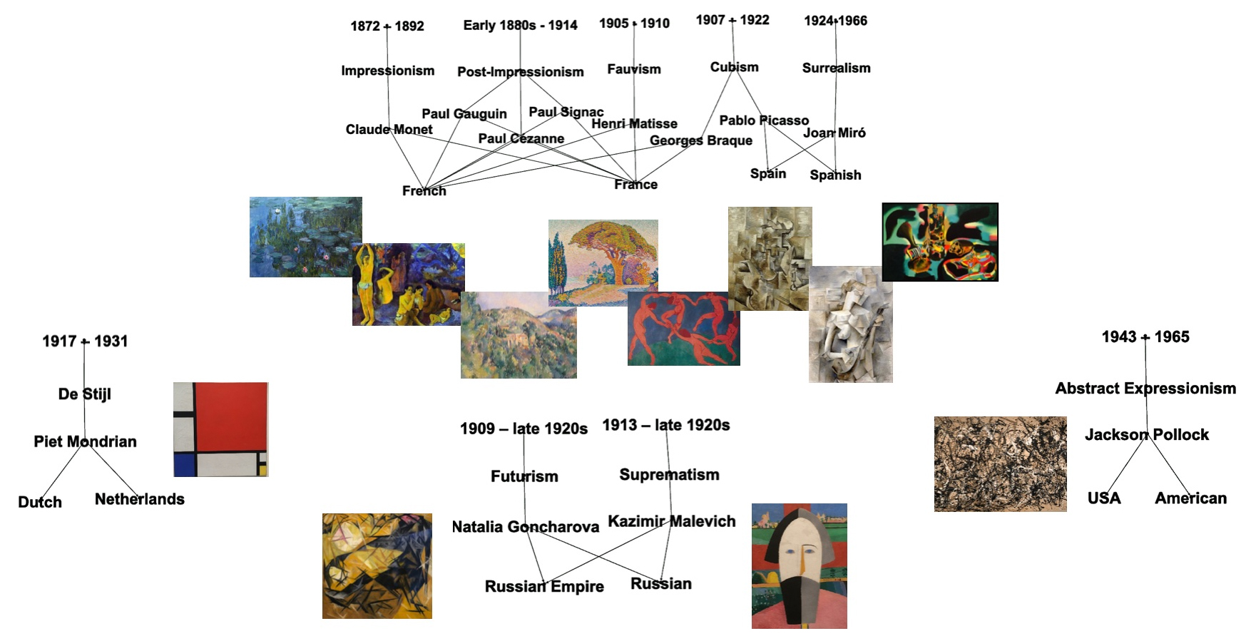
As highly connected artists, we selected Pablo Picasso and Georges Braque, artists with well known strong relationships between them: both Pablo Picasso and Georges Braque were pioneers of cubism art movement.
As highly disconnected artists, we selected Claude Monet and Kazimir Male- vich who were notably distant from each other: they lived in different time peri- ods, resided in separate countries, and belonged to contrasting art movements: Claude Monet was a key artist of impressionism and Kazimir Malevich a key artist of Suprematism. For a more detailed exploration of the relationships between modern art artists discovered through knowledge graph techniques, you can refer to our post: "Knowledge Graph for Data Integration".Transform Text Document to Semantic Graph
For each selected Wikipedia article we transformed text to semantic graphs by the following steps:- Tokenize Wikipedia text and excluded stop words.
- Generate nodes as co-located word pairs.
- Calculate edges as joint pairs that have common words. These edges represente word sequences and word chains within articles.
Tokenize Wikipedia text
from nltk.tokenize import RegexpTokenizer
tokenizer =RegexpTokenizer(r'[A-Za-z]+')

wikiArtWords=wikiArtists['Wiki']
  .apply(lambda x: RegexpTokenizer(r'[A-Za-z]+').tokenize(x)).reset_index()

wikiArtWords=wikiArtWords.explode(['words'])
wordStats=pd.merge(wikiArtWords,listArtists)

artistWordStats=wordStats.groupby('Artist').count()
  .sort_values('words',ascending=False)
Exclude stop words
Exclude stop words and short words woth length<4:import nltk
nltk.download('stopwords')
from nltk.corpus import stopwords
STOPWORDS = set(stopwords.words('english'))
dfStopWords=pd.DataFrame (STOPWORDS, columns = ['words'])
dfStopWords['stop']="stopWord"
stopWords=pd.merge(wikiArtWords,dfStopWords,on=['words'], how='left')
nonStopWords=stopWords[stopWords['stop'].isna()]
nonStopWords['stop'] = nonStopWords['words'].str.len()
nonStopWords=nonStopWords[nonStopWords['stop']>3]
nonStopWords['words']= nonStopWords['words'].str.lower()
nonStopWords.reset_index(drop=True, inplace=True)
nonStopWords['idxWord'] = nonStopWords.indexGenerated nodes as co-located word pairs
Get pairs of co-located words:bagOfWords=pd.DataFrame(nonStopWordsSubset['words'])
bagOfWords.reset_index(drop=True, inplace=True)
bagOfWords['idxWord'] = bagOfWords.index
indexWords = pd.merge(nonStopWordsSubset,bagOfWords, on=['words','idxWord'])
idxWord1=indexWords
.rename({'words':'word1','idxArtist':'idxArtist1','idxWord':'idxWord1'}, axis=1)
idxWord2=indexWords
.rename({'words':'word2','idxArtist':'idxArtist2','idxWord':'idxWord2'}, axis=1)
leftWord=idxWord1.iloc[:-1,:]
leftWord.reset_index(inplace=True, drop=True)
rightWord = idxWord2.iloc[1: , :].reset_index(drop=True)
pairWords=pd.concat([leftWord,rightWord],axis=1)
pairWords = pairWords.drop(pairWords[pairWords['idxArtist1']!=pairWords['idxArtist2']].index)
pairWords.reset_index(drop=True, inplace=True)cleanPairWords = pairWords
cleanPairWords = cleanPairWords.drop_duplicates(
subset = ['idxArtist1', 'word1', 'word2'], keep = 'last').reset_index(drop = True)
cleanPairWords['wordpair'] =
cleanPairWords["word1"].astype(str) + " " + cleanPairWords["word2"].astype(str)
cleanPairWords['nodeIdx']=cleanPairWords.indexCalculated edges as joint pairs that have common words.
Index data:nodeList1=nodeList
.rename({'word2':'theWord','wordpair':'wordpair1','nodeIdx':'nodeIdx1'}, axis=1)
nodeList2=nodeList
.rename({'word1':'theWord','idxArtist1':'idxArtist2','wordpair':'wordpair2',
'nodeIdx':'nodeIdx2'}, axis=1)
allNodes=pd.merge(nodeList1,nodeList2,on=['theWord'], how='inner')Input Data Preparation
Transform Text to Vectors
As mentioned above, for text to vector translation we used ’all- MiniLM-L6- v2’ transformer model from Hugging Face. Get unique word pairs for embeddingbagOfPairWords=nodeList
bagOfPairWords = bagOfPairWords.drop_duplicates(subset='wordpair')
bagOfPairWords.reset_index(inplace=True, drop=True)
bagOfPairWords['bagPairWordsIdx']=bagOfPairWords.indexmodel = SentenceTransformer('all-MiniLM-L6-v2')
wordpair_embeddings = model.encode(cleanPairWords["wordpair"],convert_to_tensor=True)Prepare Input Data for GNN Graph Classification Model
In GNN graph classification, the input to the model is typically a set of small graphs that represent entities in the dataset. These graphs are composed of nodes and edges, where nodes represent entities, and edges represent the relationships between them. Both nodes and edges may have associated features that describe the attributes of the entity or relationship, respectively. These features can be used by the GNN model to learn the patterns and relationships in the data, and classify or predict labels for the graphs. By considering the structure of the data as a graph, GNNs can be particularly effective in capturing the complex relationships and dependencies between entities, making them a useful tool for a wide range of applications. To prepare the input data for the GNN graph classification model, we generated labeled semantic subgraphs from each document of interest. These subgraphs were constructed by selecting neighbors and neighbors of neighbors around specific ”central” nodes. The central nodes were determined by identifying the top 500 nodes with the highest betweenness centrality within each document. By focusing on these central nodes and their neighboring nodes, we aimed to capture the relevant information and relationships within the document. This approach allowed us to create labeled subgraphs that served as the input data for the GNN graph classification model, enabling us to classify and analyze the documents effectively.import networkx as nx
list1 = [3]
list2 = [6]
radius=2
datasetTest=list()
datasetModel=list()
dfUnion=pd.DataFrame()
seeds=[]
for artist in list1 + list2:
if artist in list1:
label=0
if artist in list2:
label=1
edgeInfo0=edgeInfo[edgeInfo['idxArtist']==artist]
G=nx.from_pandas_edgelist(edgeInfo0, "wordpair1", "wordpair2")
betweenness = nx.betweenness_centrality(G)
sorted_nodes = sorted(betweenness, key=betweenness.get, reverse=True)
top_nodes = sorted_nodes[:500]
dfTopNodes=pd.DataFrame(top_nodes,columns=['seedPair'])
dfTopNodes.reset_index(inplace=True, drop=True)
for seed in dfTopNodes.index:
seed_node=dfTopNodes['seedPair'].iloc[seed]
seeds.append({'label':label,'artist':artist, 'seed_node':seed_node, 'seed':seed})
foaf_nodes = nx.ego_graph(G, seed_node, radius=radius).nodes
dfFoaf=pd.DataFrame(foaf_nodes,columns=['wordpair'])
dfFoaf.reset_index(inplace=True, drop=True)
dfFoaf['foafIdx']=dfFoaf.index
words_embed = words_embeddings.merge(dfFoaf, on='wordpair')
values1=words_embed.iloc[:, 0:384]
fXValues1= values1.fillna(0).values.astype(float)
fXValuesPT1=torch.from_numpy(fXValues1)
graphSize=dfFoaf.shape[0]
# dfFoaf.tail()
oneGraph=[]
for i in range(graphSize):
pairi=dfFoaf['wordpair'].iloc[i].split(" ", 1)
pairi1 = pairi[0]
pairi2 = pairi[1]
# for j in range(i+1,graphSize):
for j in range(graphSize):
pairj=dfFoaf['wordpair'].iloc[j].split(" ", 1)
pairj1 = pairj[0]
pairj2 = pairj[1]
if ( pairi2==pairj1):
oneGraph.append({'label':label, 'artist':artist,'seed':seed,
'centralNode':seed_node, 'k1':i, 'k2':j, 'pairi':pairi, 'pairj':pairj})
dfGraph=pd.DataFrame(oneGraph)
dfUnion = pd.concat([dfUnion, dfGraph], ignore_index=True)
edge1=torch.tensor(dfGraph[['k1','k2']].T.values)
dataset1 = Data(edge_index=edge1)
dataset1.y=torch.tensor([label])
dataset1.x=fXValuesPT1
datasetModel.append(dataset1)
loader = DataLoader(datasetModel, batch_size=32)modelSize=len(dataset)
modelSize
1000Training the Model
For this study we used the code provided by PyTorch Geometric as tutorial on GCNConv graph classification models - we just slightly tuned it for our data:Randomly split data to training and tesing
import random
torch.manual_seed(12345)
percent = 0.13
sample_size = int(modelSize * percent)
train_size=int(modelSize-sample_size)
test_dataset = random.sample(dataset, sample_size)
train_dataset = random.sample(dataset, train_size)print(f'Number of training graphs: {len(train_dataset)}')
print(f'Number of test graphs: {len(test_dataset)}')
Number of training graphs: 870
Number of test graphs: 130from torch_geometric.loader import DataLoader
train_loader = DataLoader(train_dataset, batch_size=64, shuffle=True)
test_loader = DataLoader(test_dataset, batch_size=64, shuffle=False)
for step, data in enumerate(train_loader):
print(f'Step {step + 1}:')
print('=======')
print(f'Number of graphs in the current batch: {data.num_graphs}')
print(data)
print()Prepare the model:
from torch.nn import Linear
import torch.nn.functional as F
from torch_geometric.nn import GCNConv
from torch_geometric.nn import global_mean_pool

class GCN(torch.nn.Module):
    def __init__(self, hidden_channels):
        super(GCN, self).__init__()
        torch.manual_seed(12345)
        self.conv1 = GCNConv(384, hidden_channels)
        self.conv2 = GCNConv(hidden_channels, hidden_channels)
        self.conv3 = GCNConv(hidden_channels, hidden_channels)
        self.lin = Linear(hidden_channels, 2)

    def forward(self, x, edge_index, batch):
        # 1. Obtain node embeddings
        x = self.conv1(x, edge_index)
        x = x.relu()
        x = self.conv2(x, edge_index)
        x = x.relu()
        x = self.conv3(x, edge_index)
        # 2. Readout layer
        x = global_mean_pool(x, batch)  # [batch_size, hidden_channels]
        # 3. Apply a final classifier
        x = F.dropout(x, p=0.5, training=self.training)
        x = self.lin(x)
        return x
model = GCN(hidden_channels=64)
print(model)
Train the Model:
from IPython.display import Javascript
display(Javascript('''google.colab.output.setIframeHeight(0, true, {maxHeight: 300})'''))

model = GCN(hidden_channels=64)
optimizer = torch.optim.Adam(model.parameters(), lr=0.01)
criterion = torch.nn.CrossEntropyLoss()

def train():
   model.train()
   for data in train_loader:  # Iterate in batches over the training dataset.
        out = model(data.x.float(), data.edge_index, data.batch)  # Perform a single forward pass.
        loss = criterion(out, data.y)  # Compute the loss.
        loss.backward()  # Derive gradients.
        optimizer.step()  # Update parameters based on gradients.
        optimizer.zero_grad()  # Clear gradients.

def test(loader):
    model.eval()
    correct = 0
    for data in loader:  # Iterate in batches over the training/test dataset.
        out = model(data.x.float(), data.edge_index, data.batch)
        pred = out.argmax(dim=1)  # Use the class with highest probability.
        correct += int((pred == data.y).sum())  # Check against ground-truth labels.
    return correct / len(loader.dataset)  # Derive ratio of correct predictions.

for epoch in range(1, 10):
   train()
   train_acc = test(train_loader)
   test_acc = test(test_loader)
print(f'Epoch: {epoch:03d}, Train Acc: {train_acc:.4f}, Test Acc: {test_acc:.4f}')Accuracy Metrics of the Model:
As we mentioned above, the GNN graph classification model exhibits higher sensitivity for classification compared to the GNN link prediction model. In both scenarios, we trained the models for 9 epochs. Given the distinct differences between Monet and Malevich as artists, we anticipated achieving high accuracy metrics. However, the surprising outcome was obtaining perfect metrics as 1.0000 for training data and 1.0000 for testing right from the initial training step.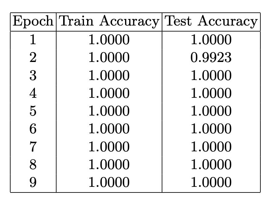 In the classification of Wikipedia articles about Pablo Picasso and Georges Braque, we were not anticipating the significant differentiation between these two documents: these artists had very strong relationships in biography and art movements. Also GNN link prediction models classified these artists as highly similar.
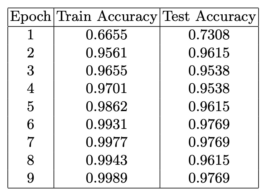 This observation highlights the high sensitivity of the GNN graph classifica- tion model and emphasizes the ability of the GNN graph classification model to capture nuanced differences and provide a more refined classification approach compared to the GNN Link Prediction models.
Model Results
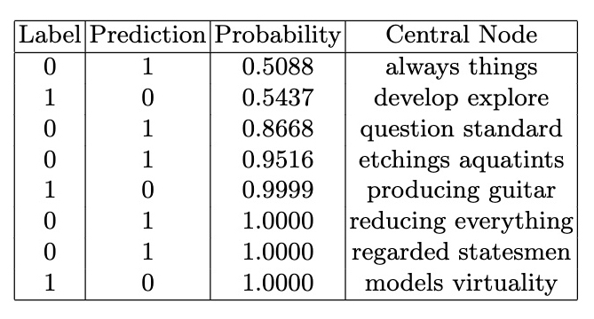
To interpret model results we calculated the softmax probabilities for each class output by the model. The softmax probabilities represent the model's confidence in its prediction for each class.modelSize
1000softmax = torch.nn.Softmax(dim = 1)
graph1=[]
for g in range(modelSize):
label=dataset[g].y[0].detach().numpy()
out = model(dataset[g].x.float(), dataset[g].edge_index, dataset[g].batch)
output = softmax(out)[0].detach().numpy()
pred = out.argmax(dim=1).detach().numpy()
graph1.append({'index':g,
'label':label,'pred':pred[0],
'prob0':round(output[0], 4),'prob1':round(output[1], 4)})