Time Series Graphs for EEG Pattern Analysis
Here we treat EEG recordings as time series graphs rather than flat lines. Each trial becomes a graph: nodes represent channels or time slices, node features store the full signal for that segment, and edges connect nodes whose activity is similar. A Graph Neural Network then learns a single fingerprint for each graph, allowing us to classify whole trials while capturing both local signal details and the relationships between them.
Because the model is highly sensitive to graph structure, small changes in how nodes connect can flip a prediction. We use this sensitivity as a tool: misclassifications and low-confidence cases highlight trials whose time series graphs do not match typical patterns. In practice, these topology-driven outliers help us spot unusual EEG behavior and point to the most interesting parts of the data for deeper analysis.
Conference & Publication
This work was presented at COMPLEX NETWORKS 2023 in Menton, France, from 28–30 November 2023, as the paper “Enhancing Time Series Analysis with GNN Graph Classification Models”. It was published in the conference proceedings with the doi: 10.1007/978-3-031-53468-3_3 .
GNN for Pattern Discovery in Time Series Data
In one of our previous posts "EEG Patterns by Deep Learning and Graph Mining" we studied how to use CNN image classification to distinguish between Alcoholic person behavior and behavior of person from Control group based on EEG data. This study was presented in "The 1st International Workshop on Time Ordered Data (ProTime2021)" of DEXA 2021 conference and it was published in "Time Series Pattern Discovery by Deep Learning and Graph Mining" paper.That study found that using the Gramian Angular Field (GAF) image transformation technique for time series data improved the accuracy of CNN image classification models compared to using raw plot pictures. By transforming the time series vectors into GAF images, the data was represented in a different embedded space that captured different aspects of the data compared to raw plots of the EEG data. This suggests that GAF image transformation is a useful technique for improving the accuracy of image classification models for time series data.
The study utilized a combination of advanced deep learning CNN image classification models and traditional graph mining techniques for time series pattern discovery. For image classification, the time series vectors were transformed into GAF images, and for graph mining, the study created graphs based on pairwise cosine similarities between the time series data points. To analyze these graphs, traditional graph mining techniques such as community detection and graph visualization were applied. This hybrid approach enabled the study to capture and analyze different aspects of the time series data, leading to a more comprehensive understanding of the patterns present in the data.
In this study we will explore how Graph Neural Network (GNN) graph classification models can be applied to classify time series data based on the underlying graph structure.
Introduction
Why GNN Graph Classification?
Graph mining is the process of extracting useful information from graphs. Traditional graph-based algorithms such as graph clustering, community detection, and centrality analysis have been used for this purpose. However, these methods have limitations in terms of their ability to learn complex representations and features from graph-structured data.
Graph Neural Networks (GNN) were developed to address these limitations. GNNs enable end-to-end learning of representations and features from graph data, allowing deep learning algorithms to process and learn from graph data. By modeling the relationships between the nodes and edges in a graph, GNNs can capture the underlying structure and dynamics of the graph. This makes them a powerful tool for analyzing and processing complex graph-structured data in various domains, including social networks, biological systems, and recommendation systems.
GNN models allow for deep learning on graph-structured data by modeling entity relationships and capturing graph structures and dynamics. They can be used for tasks such as node classification, link prediction, and graph classification. Node classification models predict the label or category of a node based on its local and global neighborhood structure. Link prediction models predict whether a link should exist between two nodes based on node attributes and graph structure. Graph classification models classify entire graphs into different categories based on their structure and attributes.
GNN graph classification models are developed to classify small graphs and in practice they are commonly used in the fields of chemistry and medicine. For example, chemical molecular structures can be represented as graphs, with atoms as nodes, chemical bonds as edges, and graphs labeled by categories.
In this post we will experiment with time series graph classification from healthcare domains and GNN graph classification models will be applied to electroencephalography (EEG) signal data by modeling the brain activity as a graph. Methods presented on this post can also be applied to time series data in various fields such as engineering, healthcare, and finance. The input data for the GNN graph classification models is a set of small labeled graphs, where each graph represents a group of nodes corresponding to time series and edges representing some measures of similarities or correlations between them.
Why EEG Data?
EEG tools studying human behaviors are well described in Bryn Farnsworth's blog "EEG (Electroencephalography): The Complete Pocket Guide". There are several reasons why EEG is an exceptional tool for studying the neurocognitive processes:
- EEG has very high time resolution and captures cognitive processes in the time frame in which cognition occurs.
- EEG directly measures neural activity.
- EEG is inexpensive, lightweight, and portable.
- EEG data is publically available: we found this dataset in Kaggle.com
The study will use the same approach as the one described above, where EEG signal data is modeled as a graph to represent brain activity. The nodes in the graph will represent brain regions or electrode locations, and edges will represent functional or structural connections between them. The raw data for the experiments will come from the kaggle.com EEG dataset 'EEG-Alcohol', which was part of a large study on EEG correlates of genetic predisposition to alcoholism.
The study aims to use GNN graph classification models to predict alcoholism, where a single graph corresponds to one brain reaction on a trial. Time series graphs will be created for each trial using electrode positions as nodes, EEG channel signals as node features, and graph edges as pairs of vectors with cosine similarities above certain thresholds. The EEG graph classification models will be used to determine whether a person is from the alcoholic or control group based on their trial reactions, which can potentially help in early detection and treatment of alcoholism.
Related Work
Machine Learning as EEG Analysis
Electroencephalography (EEG) signals are complex and require extensive training and advanced signal processing techniques for proper interpretation. Deep learning has shown promise in making sense of EEG signals by learning feature representations from raw data. In the meta-data analysis paper "Deep learning-based electroencephalography analysis: a systematic review" the authors conduct a meta-analysis of EEG deep learning and compare it to traditional EEG processing methods to determine which deep learning approaches work well for EEG data analysis and which do not.
In a previous study, EEG channel data was transformed into graphs based on pairwise cosine similarities. These graphs were analyzed using connected components and visualization techniques. Traditional graph mining methods were used to find explicit EEG channel patterns by transforming time series into vectors, constructing graphs based on cosine similarity, and identifying patterns using connected components.
Methods
In GNN graph classification for EEG data, separate graphs will be created for each brain-trial. Indicators of the alcohol or control group of corresponding person will be used as labels for the graphs. The electrode positions will be used as nodes, and channel signals will be used as node features. Graph edges will be defined as pairs of vectors with cosine similarities higher than thresholds. For the GNN graph classification model, a GCNConv (Graph Convolutional Network Convolution) model from PyTorch Geometric Library (PyG) will be used.In this section we will describe data processing and model training methods is the following order:
- Cosine similarity matrix functions.
- Process of transforming cosine similarity matrices to graphs.
- Process of training GNN graph classification model.
Cosine Similarity Function
For cosine similarities we used the following functions:
import torch
def pytorch_cos_sim(a: Tensor, b: Tensor):
    return cos_sim(a, b)
def cos_sim(a: Tensor, b: Tensor):
    if not isinstance(a, torch.Tensor):
        a = torch.tensor(a)
    if not isinstance(b, torch.Tensor):
        b = torch.tensor(b)
    if len(a.shape) == 1:
        a = a.unsqueeze(0)
    if len(b.shape) == 1:
        b = b.unsqueeze(0)
    a_norm = torch.nn.functional.normalize(a, p=2, dim=1)
    b_norm = torch.nn.functional.normalize(b, p=2, dim=1)
    return torch.mm(a_norm, b_norm.transpose(0, 1))
Cosine Similarity Matrices to Graphs
Next, for each brain-trial we will calculate cosine similarity matrices and transform them into graphs by taking only vector pairs with cosine similarities higher than a threshold.
For each brain-trial graph we will add a virtual node to transform disconnected graphs into single connected components. This process makes it is easier for GNN graph classification models to process and analyze the relationships between nodes.
Train the Model
The GNN graph classification model is designed to process input graph data, including both the edges and node features, and is trained on graph-level labels. In this case, the input data structure consists of the following components:
- Edges: The graph adjacency matrix represents the relationships between nodes in the graph. For instance, it could represent the correlations between daily temperature vectors over different years.
- Nodes with embedded features: The node features, such as the average values of the consecutive yearly sequences, would be embedded into the nodes to provide additional information to the GNN graph classification model.
- Labels on graph level: The labels, such as alcohol or control group, are assigned to the graph as a whole, and the GNN graph classification model uses these graph-level labels to make predictions about the alcohol or non-alcohol patterns.
This study uses a GCNConv model from PyTorch Geometric Library as a GNN graph classification model. The GCNConv model is a type of graph convolutional network that applies convolutional operations to extract meaningful features from the input graph data (edges, node features, and the graph-level labels). The code for the model is taken from a PyG tutorial.
Experiments
EEG Data Source
For this post we used EEG dataset that we found in kaggle.com website: 'EEG-Alcohol' Kaggle dataset. This dataset came from a large study of examining EEG correlates of genetic predisposition to alcoholism. We will classify EEG channel time series data to alcoholic and control person's EEG channels. Note: there are some data quality problems in this dataset.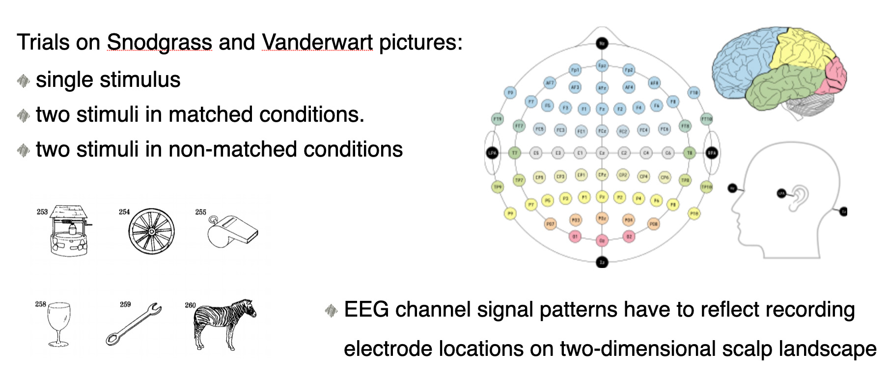 Amount of subjects in each group is 8. The 64 electrodes were placed on subject's scalps to measure the electrical activity of the brain. The response values were sampled at 256 Hz (3.9-msec epoch) for 1 second.
Each subject was exposed to either a single stimulus (S1) or to two stimuli (S1 and S2) which were pictures of objects chosen from the 1980 Snodgrass and Vanderwart picture set. When two stimuli were shown, they were presented in either a matched condition where S1 was identical to S2 or in a non-matched condition where S1 differed from S2. The total number of person-trial combination was 61.
Amount of subjects in each group is 8. The 64 electrodes were placed on subject's scalps to measure the electrical activity of the brain. The response values were sampled at 256 Hz (3.9-msec epoch) for 1 second.
Each subject was exposed to either a single stimulus (S1) or to two stimuli (S1 and S2) which were pictures of objects chosen from the 1980 Snodgrass and Vanderwart picture set. When two stimuli were shown, they were presented in either a matched condition where S1 was identical to S2 or in a non-matched condition where S1 differed from S2. The total number of person-trial combination was 61.
Transform Raw Data to EEG Channel Time Series
Kaggle EEG dataset was well analyzed in 'EEG Data Analysis: Alcoholic vs Control Groups' Kaggle notebook by Ruslan Klymentiev. We used his code for some parts of our data preparation. Here is raw data: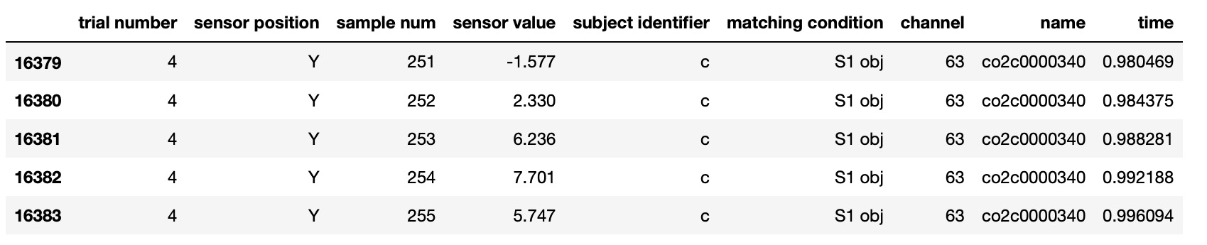 Python code to transform raw data to EEG channel time series data :
EEG_data['rn']=EEG_data.groupby(['sensor position','trial number',
   'subject identifier','matching condition','name']).cumcount()
EEG_TS=EEG_data.pivot_table(index=['trial number','sensor position',
    'subject identifier','matching condition','name','channel'],
    columns='rn',values='sensor value', aggfunc='first').reset_index()
EEG_TS.tail()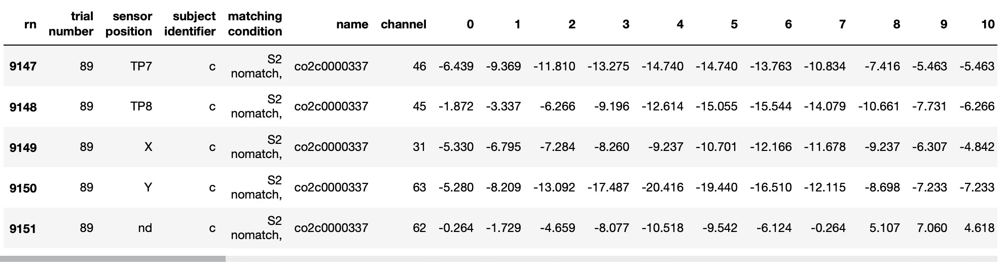
EEG_TS=EEG_TS.rename(columns={'trial number':'trial','sensor position':'position',
                                'subject identifier':'type','matching condition':'match',
'Unnamed: 0':'index'})positions=pd.DataFrame(EEG_TS['position'].unique(), columns=['position'])
positions.reset_index(drop=True, inplace=True)
positions['positionIdx']=positions.index
inputData=EEG_TS.merge(positions, on='position', how='inner')
inputData.tail()inputData = inputData.sort_values(['name', 'trial','position'])
inputData['type'] = inputData['type'].apply(lambda x: 0 if x == 'a' else 1)
inputData.reset_index(drop=True, inplace=True)
inputData['index'] = inputData.index
import math
inputData['group']=inputData['index']//61IMG='/content/drive/My Drive/EEG/groupCos/'
for group in range(0,61):
data1=inputData[(inputData['group']==group)]
values1=data1.iloc[:, 6:262]
fXValues1= values1.fillna(0).values.astype(float)
fXValuesPT1=torch.from_numpy(fXValues1)
cosine_scores1 = pytorch_cos_sim(fXValuesPT1, fXValuesPT1)
cosPairs1=[]
for i in range(61):
position1=data1.iloc[i]['position']
for j in range(61):
if i!=j:
score=cosine_scores1[i][j].detach().numpy()
position2=data1.iloc[j]['position']
combo=str(group)+'~'+position1+'~'+position2
cosPairs1.append({'combo':combo, 'left':position1, 'right':position2, 'cos': score})
dfCosPairs1=pd.DataFrame(cosPairs1)
path=IMG+str(group)+"scores.csv"
dfCosPairs1.to_csv(path, index=False)Prepare Input Data for GNN Graph Classification Model
In GNN graph classification, the input to the model is typically a set of small graphs that represent entities in the dataset. These graphs are composed of nodes and edges, where nodes represent entities, and edges represent the relationships between them. Both nodes and edges may have associated features that describe the attributes of the entity or relationship, respectively. These features can be used by the GNN model to learn the patterns and relationships in the data, and classify or predict labels for the graphs. By considering the structure of the data as a graph, GNNs can be particularly effective in capturing the complex relationships and dependencies between entities, making them a useful tool for a wide range of applications. As input for GNN graph classification for EEG data we created separate graphs for all 61 person-trial combinations. As graph labels we used indicators of alcohol or control group of corresponding person. For graph nodes as node features we used electrode positions as nodes and EEG channel signals. As graph edges, for each graph we calculated cosine similarity matrices and selected pairs of nodes with cosine similarities higher that thresholds. In this study, one of the challenges was to define thresholds for creating input graphs for GNN graph classification. As there were only 61 person-trial graphs available, this number was not sufficient for training a GNN graph classification model. To overcome this challenge, additional input graphs were created by varying the threshold values randomly within a predefined range (0.75, 0.95). This approach helped to augment the input dataset and improve the performance of the GNN graph classification model. The following code prepares input data for GNN graph classification model:- Transform cosine similarity matries to graph adjacency matrices based on treasholds
- For each brain-trial graph add a virtual node to transform disconnected graphs into single connected components.
- Transform data to PyTorch Geometric data format
import torch
import random
from torch_geometric.loader import DataLoader
datasetModel=list()
datasetTest=list()
cosPairsUnion=pd.DataFrame()
for j in range(17):
  cosPairsRange=pd.DataFrame()
  cos=round(random.uniform(0.75, 0.95), 20)
  for group in range(61):
    name=groupAtrbts.loc[group, 'name']
    trial=groupAtrbts.loc[group, 'trial']
    label=groupAtrbts.loc[group, 'type']
    data1=subData[(subData['group']==group)]
    values1=data1.iloc[:, 6:262]
    fXValues1= values1.fillna(0).values.astype(float)
    fXValuesPT1=torch.from_numpy(fXValues1)
    fXValuesPT1avg=torch.mean(fXValuesPT1,dim=0).view(1,-1)
    fXValuesPT1union=torch.cat((fXValuesPT1,fXValuesPT1avg),dim=0)
    cosPairs1=[]
    for i in range(61):
      position1='XX'
      position2=positionList[(positionList['positionIdx']==i)]['position']
      cosPairs1.append({'round':j, 'cos':cos,
          'group':group, 'label':label, 'k1':61,'k2':i,
          'pos1':position1, 'pos2':position2,'score': 0.99})
    edge1=edges[(edges['group']==group)]
    edge1.reset_index(drop=True, inplace=True)
    edge1['index'] = edge1.index
    size=edge1.shape[0]
    for i in range(size):
      score2=edge1.loc[i, 'cos']
      if score2>cos:
        position1=edge1['col1'][i]
        position2=edge1['col2'][i]
        k1= positionList['positionIdx'].index[positionList['position'] == position1][0]
        k2= positionList['positionIdx'].index[positionList['position'] == position2][0]
        cosPairs1.append({'round':j, 'cos':cos,
            'group':group, 'label':label, 'k1':k1,'k2':k2,
            'pos1':position1, 'pos2':position2,'score': score2})
    dfCosPairs1=pd.DataFrame(cosPairs1)
    edge2=torch.tensor(dfCosPairs1[['k1','k2']].T.values)
    dataset1 = Data(edge_index=edge2)
    dataset1.y=torch.tensor([label])
    dataset1.x=fXValuesPT1union
    datasetModel.append(dataset1)
    loader = DataLoader(datasetModel, batch_size=32)
    cosPairsRange = cosPairsRange.append([dfCosPairs1])
    cosPairsUnion = cosPairsUnion.append([dfCosPairs1])
modelSize=len(dataset)
modelSize
1037
Training GNN Graph Classification Model
Randomly split input data to training and tesing:import random
torch.manual_seed(12345)
percent = 0.15
sample_size = int(modelSize * percent)
train_size=int(modelSize-sample_size)
test_dataset = random.sample(dataset, sample_size)
train_dataset = random.sample(dataset, train_size)e)
test_loader = DataLoader(test_dataset, batch_size=32, shuffle=True)from torch.nn import Linear
import torch.nn.functional as F
from torch_geometric.nn import GCNConv
from torch_geometric.nn import global_mean_pool
class GCN(torch.nn.Module):
def __init__(self, hidden_channels):
super(GCN, self).__init__()
torch.manual_seed(12345)
self.conv1 = GCNConv(256, hidden_channels)
self.conv2 = GCNConv(hidden_channels, hidden_channels)
self.conv3 = GCNConv(hidden_channels, hidden_channels)
self.lin = Linear(hidden_channels, 2)
def forward(self, x, edge_index, batch):
# 1. Obtain node embeddings
x = self.conv1(x, edge_index)
x = x.relu()
x = self.conv2(x, edge_index)
x = x.relu()
x = self.conv3(x, edge_index)
# 2. Readout layer
x = global_mean_pool(x, batch) # [batch_size, hidden_channels]
# 3. Apply a final classifier
x = F.dropout(x, p=0.5, training=self.training)
x = self.lin(x)
return x
model = GCN(hidden_channels=64)Train the Model
from IPython.display import Javascript
display(Javascript('''google.colab.output.setIframeHeight(0, true, {maxHeight: 300})'''))
model = GCN(hidden_channels=64)
optimizer = torch.optim.Adam(model.parameters(), lr=0.01)
criterion = torch.nn.CrossEntropyLoss()
def train():
model.train()
for data in train_loader: # Iterate in batches over the training dataset.
out = model(data.x.float(), data.edge_index, data.batch) # Perform a single forward pass.
loss = criterion(out, data.y) # Compute the loss.
loss.backward() # Derive gradients.
optimizer.step() # Update parameters based on gradients.
optimizer.zero_grad() # Clear gradients.
def test(loader):
model.eval()
correct = 0
for data in loader: # Iterate in batches over the training/test dataset.
out = model(data.x.float(), data.edge_index, data.batch)
pred = out.argmax(dim=1) # Use the class with highest probability.
correct += int((pred == data.y).sum()) # Check against ground-truth labels.
return correct / len(loader.dataset) # Derive ratio of correct predictions.
for epoch in range(1, 10):
train()
train_acc = test(train_loader)
test_acc = test(test_loader)
print(f'Epoch: {epoch:03d}, Train Acc: {train_acc:.4f}, Test Acc: {test_acc:.4f}')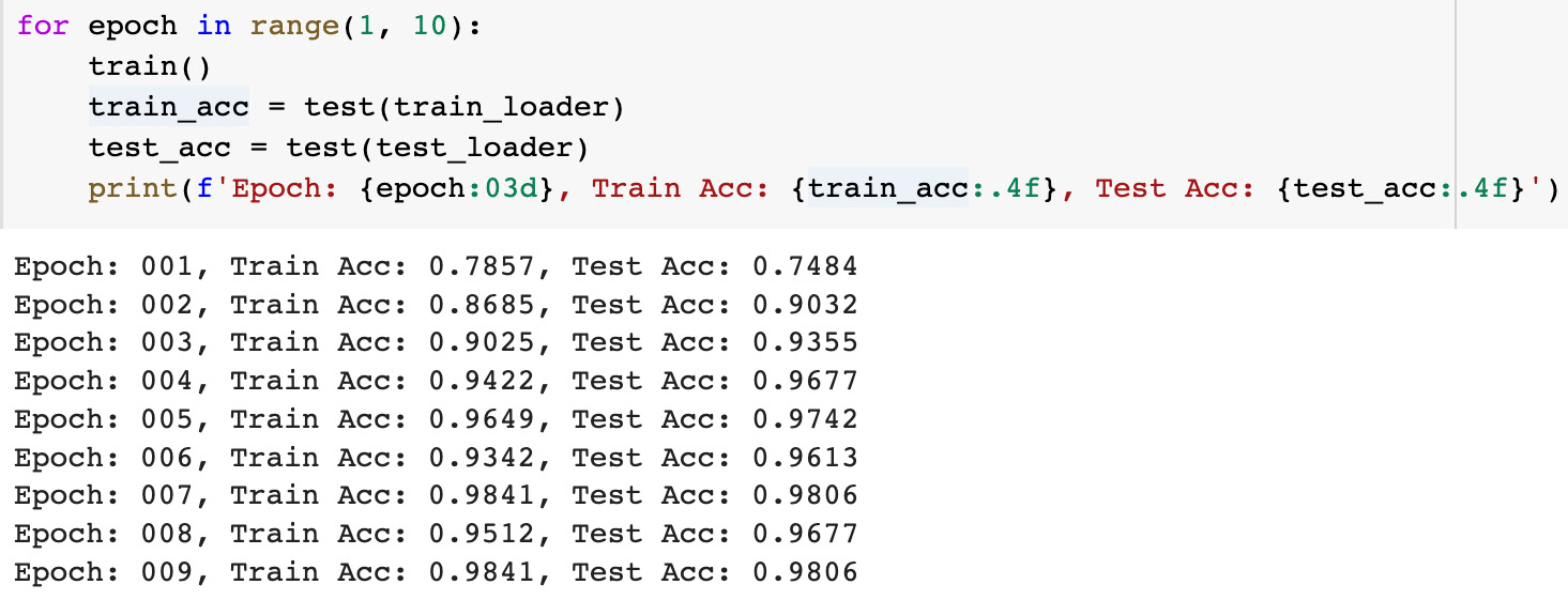 To estimate the model results we used the same model accuracy metrics as in the PyG tutorial: training data accuracy was about 98.4 percents and testing data accuracy was about 98.1 percents. Reasons for the fluctations in accuracy can be explained by the rather small dataset (only 155 test graphs)
Interpret EEG Model Results
To interpret model results we calculated the softmax probabilities for each class output by the model. The softmax probabilities represent the model's confidence in its prediction for each class. In the output of the graph classification model we have 17 outliers with the model's predictions not equal to the input labels.modelSize
1037softmax = torch.nn.Softmax(dim = 1)
graph1=[]
for g in range(modelSize):
label=datasetTest[g].y[0].detach().numpy()
out = model(datasetTest[g].x.float(), datasetTest[g].edge_index, datasetTest[g].batch)
output = softmax(out)[0].detach().numpy()
pred = out.argmax(dim=1).detach().numpy()
graph1.append({'index':g,
'label':label,'pred':pred[0],
'prob0':round(output[0], 4),'prob1':round(output[1], 4)})graph2df=pd.DataFrame(graph1)
len(graph2_df[graph2_df['label']==graph2_df['pred']])
1020
len(graph2_df[graph2_df['label']!=graph2_df['pred']])
17graphDF[graphDF['label']!=graphDF['pred']].sort_values('prob0').head(20)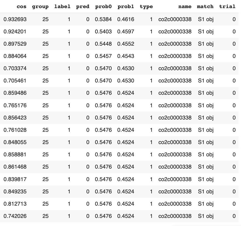 Our observations:
- Probabilities of incorrectly predicted graph classification labels is close to 0.5 (between 0.45 and 0.55), which means that the model is very uncertain about these predictions.
- Type of stimulus in all outlier graphs is "single stimulus".
- All outlier graphs belong to the same person (records have the same name, but different trials). These graphs marked as persons from Control group but they were predicted as persons from Alchogol group.
Most of graph classifiction model results with low confidence also are related to "single stimulus" patters:
graphDF['diff']=abs(graphDF['prob1']-graphDF['prob0'])
graphDF.sort_values('diff').head(24)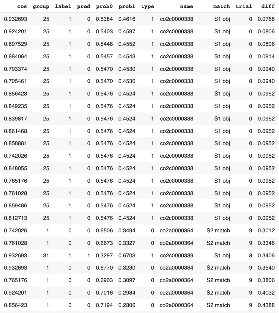 This corresponds with the results of our previous study about EEG signal classification:
trials with "single stimulus" patters had lower confidence on CNN time series classification compared to trials with "two stimuli, matched" and "two stimuli, non-matched" patterns.
This corresponds with the results of our previous study about EEG signal classification:
trials with "single stimulus" patters had lower confidence on CNN time series classification compared to trials with "two stimuli, matched" and "two stimuli, non-matched" patterns.
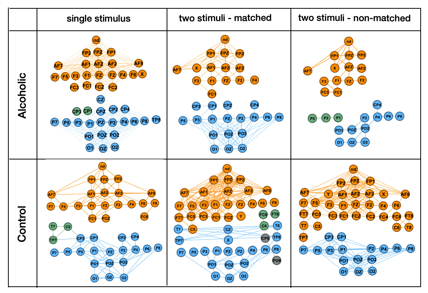
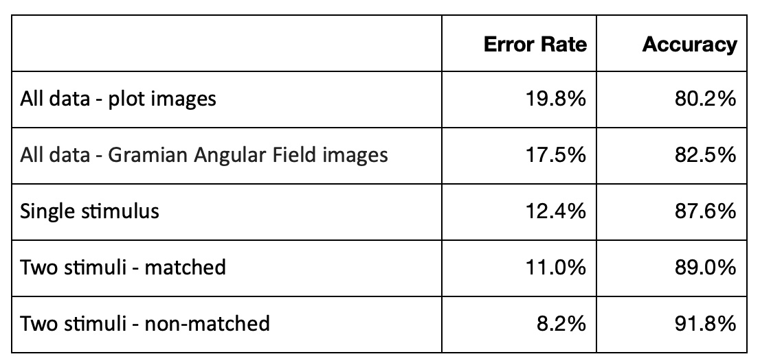 More interesting, graph vizualiation examples show that trials with "single stimulus" patters have much lower differences between persons from Alcoholic and Control groups then trials with "two stimuli, matched" and "two stimuli, non-matched" patterns.
The results of a previous study showed that trials with "single stimulus" patterns had much lower differences between persons from the alcoholic and control groups compared to trials with "two stimuli, matched" and "two stimuli, non-matched" patterns. This suggests that "single stimulus" trials are not sufficient for accurately distinguishing between the two groups. Furthermore, graph visualization examples taken from the previous study demonstrated this difference in patterns between the different types of stimuli.
More interesting, graph vizualiation examples show that trials with "single stimulus" patters have much lower differences between persons from Alcoholic and Control groups then trials with "two stimuli, matched" and "two stimuli, non-matched" patterns.
The results of a previous study showed that trials with "single stimulus" patterns had much lower differences between persons from the alcoholic and control groups compared to trials with "two stimuli, matched" and "two stimuli, non-matched" patterns. This suggests that "single stimulus" trials are not sufficient for accurately distinguishing between the two groups. Furthermore, graph visualization examples taken from the previous study demonstrated this difference in patterns between the different types of stimuli.
Conclusion
In conclusion, this study provides evidence that GNN graph classification models can effectively classify time series data represented as graphs in EEG data. The study found that these methods are capable of capturing the complex relationships between the nodes in the input graphs and use this information to accurately classify them. For each person-trial we created separate graphs that were labeled according to whether the corresponding person belonged to the alcohol or control group. Graph nodes were represented by electrode positions and node features were represented by the EEG channel signals. Cosine similarity matrices were used to define graph edges by selecting vector pairs with cosines above a threshold, and transforming them into graph adjacency matrices. To ensure disconnected graphs became single connected components, to each graph was also added a virtual node. The study encountered a limitation in the amount of input graphs available for model training. To overcome this limit, random thresholds were used to create additional input graphs, which increased the amount of input data available for training and improved the accuracy of the predictions. The study found that GNN graph classification models are highly effective in accurately classifying time series data by capturing the relationships between the data points and using this information to make accurate predictions. In particular, GNN graph classification models accurately classified EEG recordings as alcoholic or non-alcoholic person. The study identified some interesting outliers where the GNN graph classification model had difficulty accurately predicting the results. Specifically, it found that the model struggled to accurately classify graphs with a "single stimulus" type of stimulus and "single stimulus" trials were not sufficient for accurately distinguishing between the control and alcohol groups in EEG recordings. This finding is consistent with the results of a previous study, which found that trials with "single stimulus" patterns had lower confidence in CNN time series classification compared to trials with "two stimuli, matched" and "two stimuli, non-matched" patterns. Future research could investigate the use of GNN graph classification methods for other types of time series data and explore ways to address the identified limitations of these models. Overall, we believe that GNN graph classification models have great potential for a variety of applications in fields such as healthcare, environmental monitoring, and finance. For example, stock prices can be modeled as time series data and GNN Graph classification algorithms can be used to classify groups of time series into different patterns, such as bullish or bearish trends, which can be used for predicting future prices. We hope that our study will contribute to the development of more accurate and effective classification models for time series data domains.