Link Prediction for Knowledge Graphs
In our previous post 'Knowledge Graph for Data Mining' we discussed knowledge graph building and mining techniques. These techniques were presented in 2020 in DEXA conference "Machine Learning and Knowledge Graphs" workshop and published as 'Building Knowledge Graph in Spark without SPARQL' paper.
The goal of that study was to demonstrate that knowledge graph area is much wider that traditional semantic web SPARQL approach and there are non-traditional ways to build and explore knowledge graphs. In that study we demonstrated how knowledge graph techniques can be accomplished by Spark GraphFrames library. In this study we will show other techniques that can be applied to creating and rewiring knowledge graphs. We will explore building knowledge graphs based on Wikipedia data and Graph Neural Networks (GNN) link prediction model. To compare results of this study with results of our previous study we will use data about the same list of modern art artists.Introduction: Knowledge Graphs Exploration
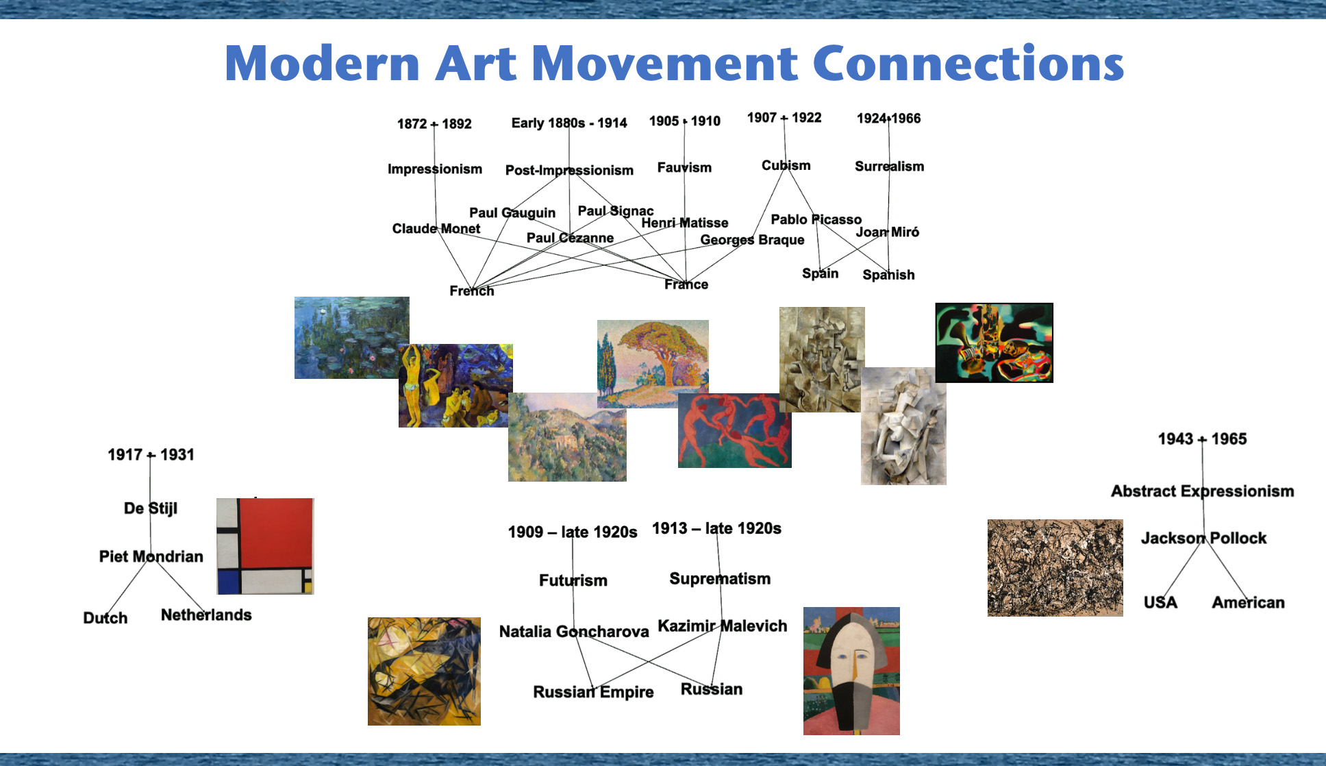
In recent years knowledge graph becomes more and more popular for data mining. DEXA conference is well known for data mining and in 2020 they organized the first "Machine Learning and Knowledge Graphs" workshop. In that workshop we presented a paper where we showed how to build knowledge graph in Spark without SPARQL and how conceptually knowledge graph builds a bridge between logical thinking and graph thinking for data mining. As a data source for that study we used data about paintings of several artists from MoMA collection taken from kaggle dataset 'Museum of Modern Art Collection'. Through knowledge graph we explored how artists were conneted and how they influensed each other: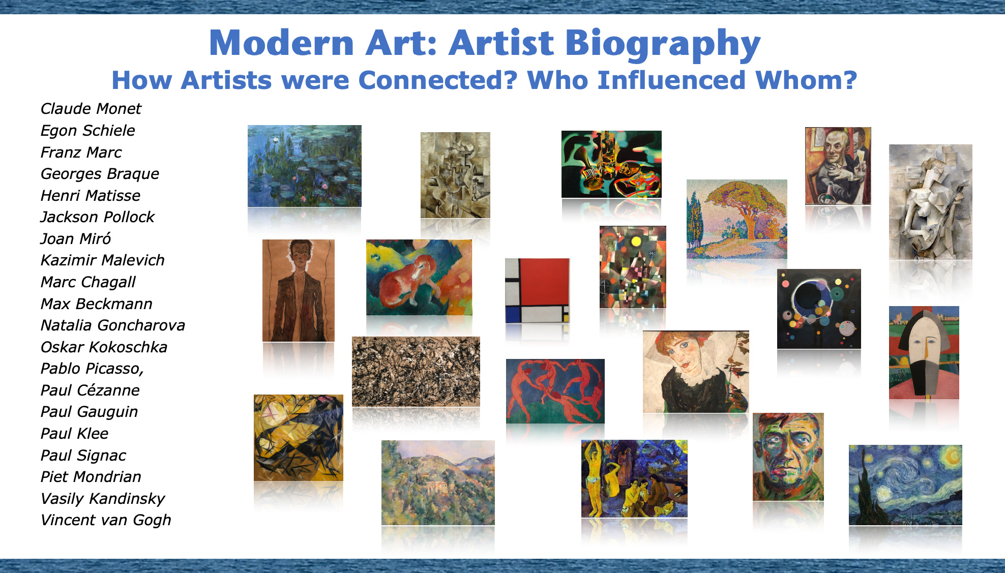 In that study we explored knowledge graph using Spark DataFrames library techniques and found unknown connections between artists and between modern art movements.
 In this post as data source we will use Wikipedia text data about the same 20 artists that we used in the previous study and we will investigate semantic connections between the artists through GNN link prediction model.
Methods
To find connections between the artists we will do the following:- Build a graph with artist names and Wikipedia text as nodes and connections between artist names and corresponding Wikipedia articles as edges.
- Embed node text to vectors by transformers model.
- Analyze cosine similarity matrix for transformer embedded nodes and add graph edges for artist pairs with high cosine similarities.
- On top of this graph run GNN link prediction model.
Building Graph
For data processing, model training and interpreting the results we will use the following steps:- Tokenize Wikipedia text to compare artist Wikipedia pages by size distribution
- Define nodes as artist names and Wikipedia articles
- Define edges as pairs of artist names and corresponding articles
- Build a knowledge graph on those nodes and edges
Transform Text to Vectors
As a method of text to vector translation we used 'all-MiniLM-L6-v2' model from Hugging Face. This is a sentence-transformers model that maps text to a 384 dimensional dense vector space.
There are two advantages of embedding text nodes:
- Vectors generated by transformers can be used for GNN link prediction model as node features
- Based on highly connected vector pairs additional graph edges can be generated.
Run GNN Link Prediction Model
As Graph Neural Networks link prediction we used a model from Deep Graph Library (DGL). The model is built on two GrapgSAGE layers and computes node representations by averaging neighbor information. We used the code provided by DGL tutorial DGL Link Prediction using Graph Neural Networks.
The results of this code are embedded nodes that can be used for further analysis such as node classification, k-means clustering, link prediction and so on. In this study we used it for link prediction by estimating cosine similarities between embedded nodes.
Find Connections
To calculate how similar are vectors to each other we will do the following:- Calculate cosine simmilarity matrix
- Demonstrate examples of highly connected and lowly connected node pairs.
Cosine Similarities function:
import torch
def pytorch_cos_sim(a: Tensor, b: Tensor):
    return cos_sim(a, b)
def cos_sim(a: Tensor, b: Tensor):
    if not isinstance(a, torch.Tensor):
        a = torch.tensor(a)
    if not isinstance(b, torch.Tensor):
        b = torch.tensor(b)
    if len(a.shape) == 1:
        a = a.unsqueeze(0)
    if len(b.shape) == 1:
        b = b.unsqueeze(0)
    a_norm = torch.nn.functional.normalize(a, p=2, dim=1)
    b_norm = torch.nn.functional.normalize(b, p=2, dim=1)
    return torch.mm(a_norm, b_norm.transpose(0, 1))
Experiments
Data Source Analysis
As data source we used text data from Wikipedia articles about the same 20 artists that we used in the previous study "Building Knowledge Graph in Spark without SPARQL". In that study coding was done in Scala Spark and in this study coding was done in Python. As envinroment we used Google Colab and Google Drive.To estimate the size distribution of Wikipedia text data we tokenized the text and exploded the tokens:
from nltk.tokenize import RegexpTokenizer
tokenizer = RegexpTokenizer(r'\w+')

wikiArtWords=wikiArtists['Wiki']
  .apply(lambda x: RegexpTokenizer(r'\w+').tokenize(x)).reset_index()

wikiArtWords['words']=wikiArtWords['Wiki']
wikiArtWords=wikiArtWords.rename(columns={'index': 'idxArtist'})

wikiArtWords=wikiArtWords.explode(['words'])
wikiArtWords.shape
(118167, 3)
Here is the distribution of number of words in Wikipedia related to artits:
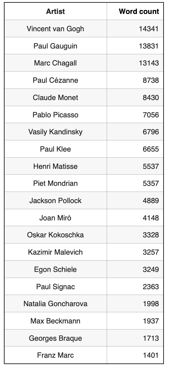
wikiArtWords.groupby('idxArtist').count().describe()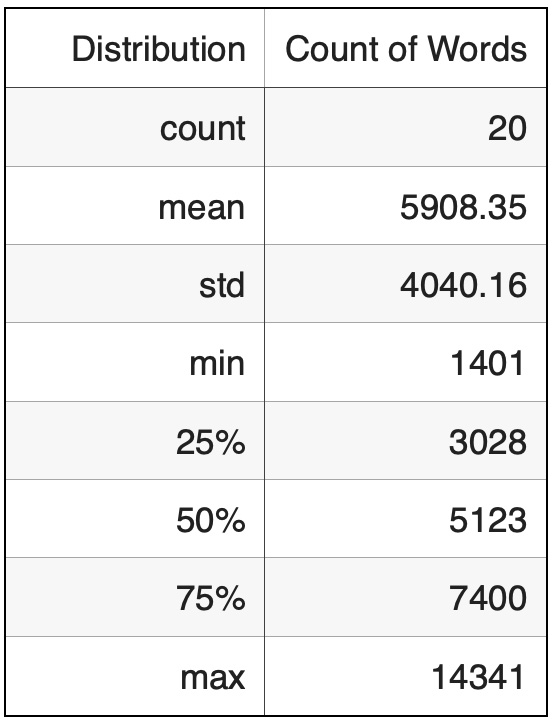
Based on Wikipedia text size distribution, the most well known artist in our artist list is Vincent van Gogh and the most unknown artist is Franz Marc.
Building Graph
Index data:wikiArtists['idxArtist'] = wikiArtists.index
wikiArtists['idxWiki'] = wikiArtists.index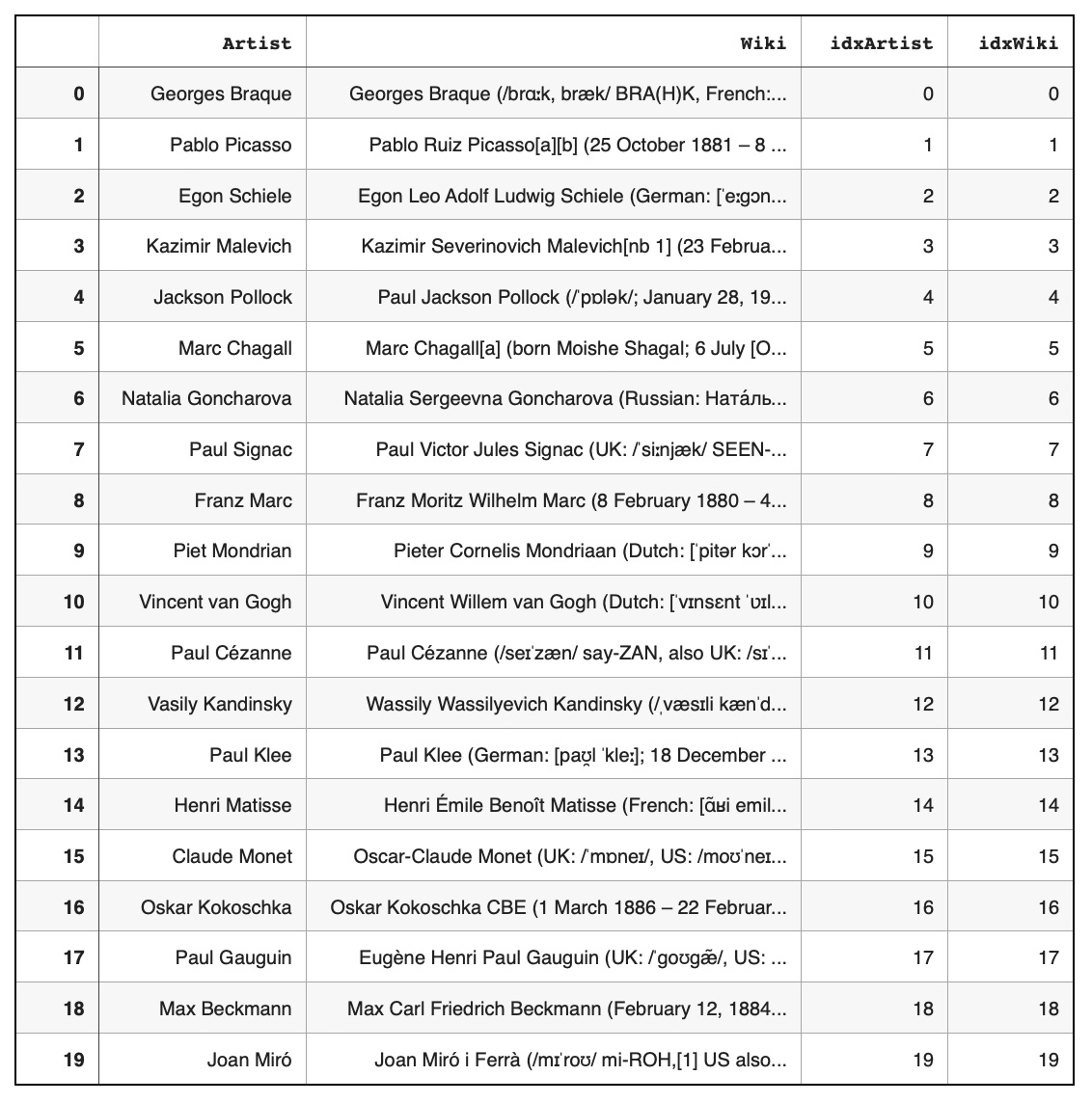 Define nodes as artist names ('Artist' column) and Wikipedia article text ('Wiki' column):
node1=wikiArtists[["Wiki","idxWiki"]]
node1.rename(columns={'Wiki':'node','idxWiki':'idx'}, inplace=True)
node2=wikiArtists[["Artist","idxArtist"]]
node2.rename(columns={'Artist':'node','idxArtist':'idx'}, inplace=True)
nodes=pd.concat([node2,node1], axis=0)
nodes = nodes.reset_index(drop=True)
nodes['idxNode']=nodes.index
nodes.shape
(40, 3)edges=nodes[['idx','idxNode']]
edges.shape
(40, 2)Transform Text to Vectors
For text to vector translation we used 'all-MiniLM-L6-v2' model from Hugging Face:model = SentenceTransformer('all-MiniLM-L6-v2')
wiki_embeddings = model.encode(nodes["node"],convert_to_tensor=True)
wiki_embeddings.shape
torch.Size([40, 384])with open(drivePath+'wiki.pkl', "wb") as fOut:
pickle.dump({'idx': nodes["idxNode"],
'words': nodes["node"],
'embeddings': wiki_embeddings.cpu()},
fOut, protocol=pickle.HIGHEST_PROTOCOL)Add Edges to the Knowledge Graph
To indicate what edges should be aded to the knowledge graph we analyzed a cosine similarity matrix and selected pairs of vectors with high cosine similarities:cos_scores_wiki=pytorch_cos_sim(wiki_embeddings,wiki_embeddings)
pairs_wiki=[]
for i in range(0, 40) :
for j in range(0, 40):
pairs_wiki.append({ 'node1':i,'node2': j,'cos': cos_scores_wiki[i][j].numpy()})
dfPairs_wiki=pd.DataFrame(pairs_wiki)
dfArtistPairs_wiki=dfPairs_wiki[(dfPairs_wiki['node1']<dfPairs_wiki['node2'])
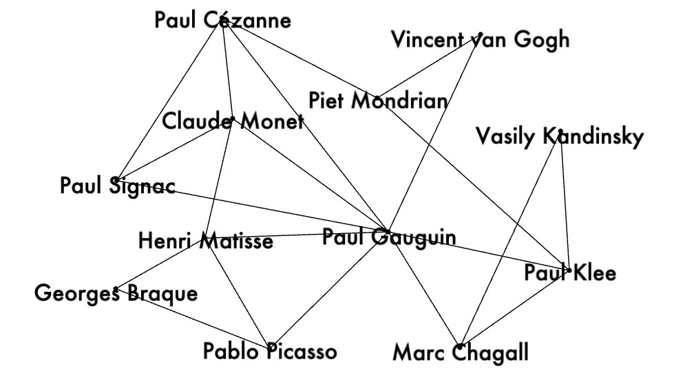
& (dfPairs_wiki['node1']>19)]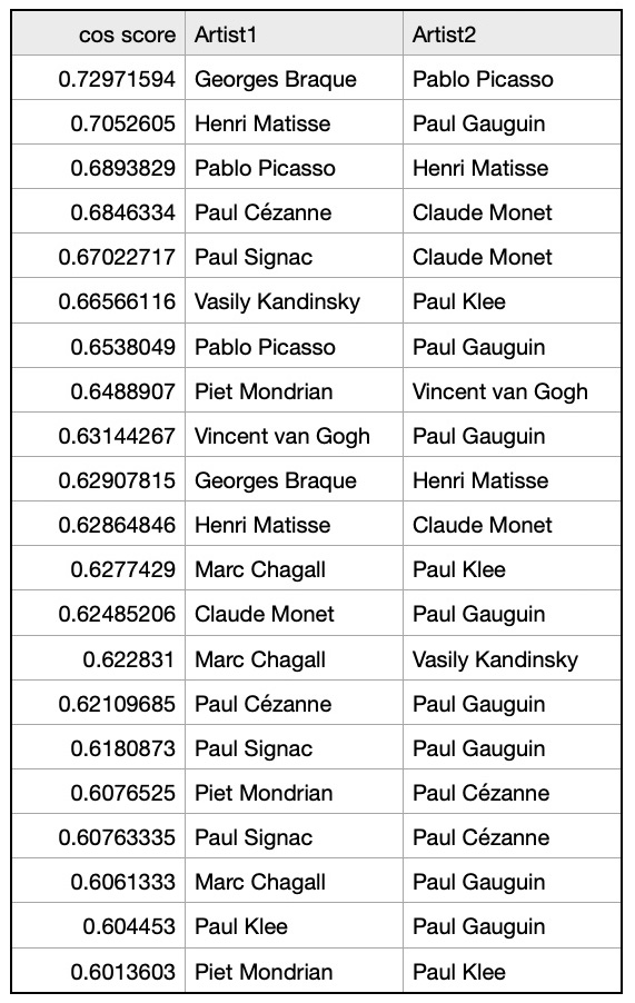 Graph on artist pairs with cosine similarities > 0.6:
 Selected edges were added to the list of graph edges and loaded to Google Drive:
edges.to_csv(drivePath+"edges.csv", index=False)Run GNN Link Prediction Model
As Graph Neural Networks (GNN) link prediction model we used a model from Deep Graph Library (DGL). The model code was provided by DGL tutorial and we only had to transform nodes and edges data from our data format to DGL data format.
Read embedded nodes and edges from Google Drive:with open(drivePath+'wiki.pkl', "rb") as fIn:
stored_data = pickle.load(fIn)
gnn_index = stored_data['idx']
gnn_words = stored_data['words']
gnn_embeddings = stored_data['embeddings']
edges=pd.read_csv(drivePath + 'edges.csv')Convert data to DGL format:
unpickEdges=edges
edge_index=torch.tensor(unpickEdges[['idx','idxNode']].T.values)
u,v=edge_index[0],edge_index[1]
g=dgl.graph((u,v))
g.ndata['feat']=gnn_embeddings
g=dgl.add_self_loop(g)
g
Graph(num_nodes=40, num_edges=101,
ndata_schemes={'feat': Scheme(shape=(384,), dtype=torch.float32)}
edata_schemes={})model = GraphSAGE(train_g.ndata['feat'].shape[1], 64)
pred = DotPredictor()
def compute_loss(pos_score, neg_score):
scores = torch.cat([pos_score, neg_score])
labels = torch.cat([torch.ones(pos_score.shape[0]), torch.zeros(neg_score.shape[0])])
return F.binary_cross_entropy_with_logits(scores, labels)
def compute_auc(pos_score, neg_score):
scores = torch.cat([pos_score, neg_score]).numpy()
labels = torch.cat(
[torch.ones(pos_score.shape[0]), torch.zeros(neg_score.shape[0])]).numpy()
return roc_auc_score(labels, scores)Knowledge Graph with Predicted Edges
To calculate predicted edges, first we looked at cosine similarity matrix for pairs of nodes embedded by GNN link prediction model:cosine_scores_gnn = pytorch_cos_sim(h, h)
pairs_gnn = []
for i in range(len(cosine_scores_gnn)):
for j in range(len(cosine_scores_gnn)):
pairs_gnn.append({'idx1': i,'idx2': j,
'score': cosine_scores_gnn[i][j].detach().numpy()})
dfArtistPairs_gnn=pd.DataFrame(pairs_gnn)
gnnPairs=dfArtistPairs_gnn[(dfArtistPairs_gnn['idx1']<dfArtistPairs_gnn['idx2'])
& (dfArtistPairs_gnn['idx1']>19)]
gnnPairs.reset_index(inplace=True)
gnnPairs['idxSort']=gnnPairs.indexgnnPairs0=gnnPairs
gnnPairs0 =gnnPairs0.drop('index', axis=1)
gnnPairs0.head(3)
idx1 idx2 score idxSort
0 35 37 0.9553253 0
1 30 35 0.9276154 1
2 20 21 0.9113796 2List of Artist Names:
listArtists.head(3)
      Artist     idxArtist
0   Georges Braque   0
1   Pablo Picasso    1
2   Egon Schiele     2
Join edge cosine similarity scores with artist names by indexes:
listArtists1=listArtists
listArtists1['idx1'] = listArtists1['idxArtist'].astype(int) + 20
listArtists1=listArtists1.rename(columns={'Artist': 'Artist1'})
listArtists1 =listArtists1.drop('idxArtist', axis=1)

listArtists2=listArtists
listArtists2['idx2'] = listArtists2['idxArtist'].astype(int) + 20
listArtists2=listArtists2.rename(columns={'Artist': 'Artist2'})
listArtists2 =listArtists2.drop('idxArtist', axis=1)

gnnPairs1=pd.merge(gnnPairs0,listArtists1,on="idx1")
gnnPairs2=pd.merge(gnnPairs1,listArtists2,on="idx2")gnnPairs2["line"]= '"'+gnnPairs2['Artist1'].astype(str) + '" -> "' + gnnPairs2['Artist2'] + '";'
gnnPairs2.show()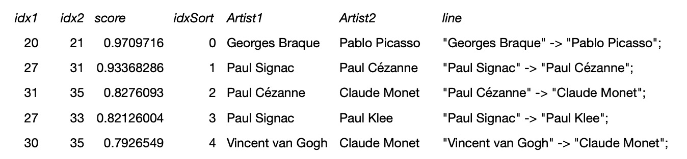 In the following examples will show graphs of artists with hign cosine similarities and low codine similarities.
Pairs of artists with high cosine similarities -- higher than 0.6:
In the following examples will show graphs of artists with hign cosine similarities and low codine similarities.
Pairs of artists with high cosine similarities -- higher than 0.6:
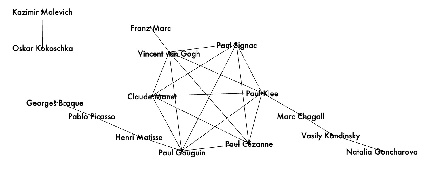
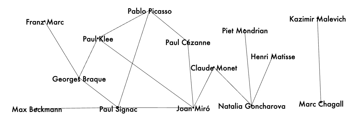
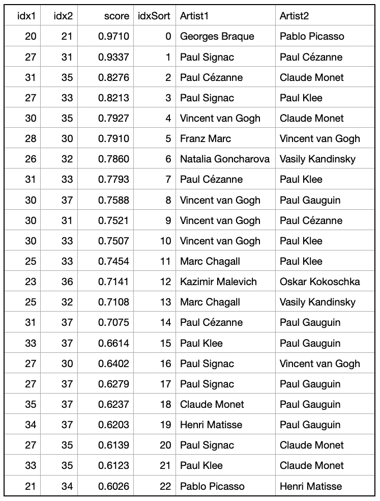 Example 1: artist pairs with cosine similarities > 0.6:
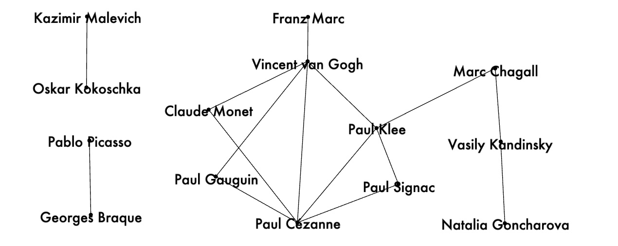
 Example 2: artist pairs with cosine similarities > 0.7:
 Pairs of artists with low cosine similarities -- less than -0.5:
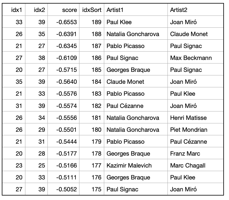 Example 3: artist pairs with cosine similarities < -0.5:
Conclusion
In this post we demonstrated how to use transformers and GNN link predictions to rewire knowledge graphs.- Trough transformers we mapped Wikipedia articles to vectors and added pairs of highly connected artists as edges to the knowledge graph.
- On top of the renovated knowledge graph we ran GNN link prediction model.
- We used cosine similarities between GNN embedded nodes to estimate knowledge graph predicted edges.
- We demonstrated how to apply these techniques to find pairs of artists that are highly connected or lowly connected.