Hidden Connectors in Knowledge Graphs
In this project, we dive into a semantic knowledge graph built from art biographies and go beyond the simple question “who is linked to whom?”. We use Graph AI to embed nodes in a vector space and measure how strongly they connect, then examine tiny three-node patterns (triangles) to find cases where one link is much stronger than the others. Those nodes often act as quiet bridges between otherwise distant concepts or artists.
The same idea scales far beyond art. In medicine, hidden connectors can illuminate critical genetic pathways that influence disease and point toward targeted therapies. In social networks, they reveal quiet influencers and emerging trends. In finance, connector analysis can surface firms that quietly support market stability; in criminal intelligence, it can highlight organizers who sit behind fragmented activity.
Conference Highlights
This research was presented at the 17th International Conference on Information Technology and Applications (ICITA 2023), held in Turin, Italy from October 20–22, 2023. The paper, “Uncovering Hidden Connections: Granular Relationship Analysis in Knowledge Graphs”, was published as Romanova, A. Uncovering Hidden Connections: Granular Relationship Analysis in Knowledge Graphs, in the ICITA 2023 proceedings, doi: 10.1007/978-981-99-8324-7_2 . To complement the text understanding, in this post we will feature some slides from the conference presentation.
Uncovering Hidden Triangles in Knowledge Graphs
In recent years, knowledge graphs have become a powerful tool for integrating and analyzing data and shedding lights on the connections between entities. This study narrows its focus on unraveling detailed relationships within knowledge graphs, placing special emphasis on the role of graph connectors through link predictions and triangle analysis.
Using Graph Neural Network (GNN) Link Prediction models and graph triangle analysis in knowledge graphs, we have managed to uncover relationships that had been previously undetected or overlooked. Our findings mark a significant milestone, paving the way for more comprehensive exploration into the complex relationships that exist within knowledge graphs.
This study initiates further research in the area of unveiling the hidden dynamics and connections in knowledge graphs. The insights from this work promise to redefine our understanding of knowledge graphs and their potential for unlocking the complexities of data interrelationships.
Introduction
Deep Learning, Knowledge Graphs and the Emergence of GNN
The year 2012 was pivotal for deep learning and knowledge graphs. In that year, after AlexNet was introduced, a Convolutional Neural Network (CNN) highlighted the power of image classification techniques. Simultaneously, Google's introduction of knowledge graphs transformed data integration and management.
For many years, deep learning and knowledge graphs developed independently. CNN proved effective with grid-structured data but struggled with graph-structured data. On the other hand, graph techniques excelled in representing and reasoning about graph data but lacked deep learning's power. The late 2010s Graph Neural Networks (GNN) bridged this gap and emerged as a potent tool for processing graph-structured data through deep learning techniques.
For years, we've relied on binary graph structures, simplifying complex relationships into 'yes' or 'no', '1' or '0'. But in our ever-evolving world, is that enough? We believed there was more depth to be explored. Thus, we turned to Graph Neural Networks, a frontier technology, to help us transition from these fixed binaries to a more fluid, continuous space.
Our Past Experiments in Rewiring of Knowledge Graphs
In our previous study 'Rewiring Knowledge Graphs by Link Predictions' we delved into the exploration of knowledge graph rewiring to reveal unknown relationships between modern art artists, employing GNN link prediction models. By training these models on Wikipedia articles about modern art artists' biographies and leveraging GNN link prediction models, we identified previously unknown relationships between artists.
To rewire knowledge graphs, we adopted two distinct methods. First, we utilized a traditional method that involved a full-text analysis of articles and calculation of cosine similarities between embedded nodes. The second method involved the construction of semantic graphs based on the distribution of pairs of co-located words, and edges between nodes that share common words.
New Study: Focusing on Graph Triangles
In this study, we continue to leverage the same data source and employ similar techniques for graph representation. However, we introduce a novel approach of comparing two documents and examining entity relationships at granular level. Specifically, we concentrate on analyzing graph triangles, where one side displays a stronger connection than the other two sides.Let's take a moment to appreciate the evolution and elevation that GNN Link Prediction brings to the table. Remember the days of black and white television? Now imagine transitioning from that to a high-definition colored TV. That's the kind of transformative leap we're talking about when moving from traditional graph representations to GNN Link Prediction. Instead of just binary relationships, we're now operating on a continuous spectrum. Why is this so revolutionary? Because it allows us to see the subtle intricacies, the patterns that were once invisible. We're no longer just categorizing relationships as 'connected' or 'not connected'; we're exploring the depth, the weight, the very essence of these connections. It's like being given a magnifying glass to see the intricate patterns that were always there but previously overlooked. This shift not only boosts our prediction accuracy but also broadens our understanding of the complex web of relationships within our data.
In the vast network of relationships, it's essential to understand not just who is connected to whom, but also the depth and nature of these connections. Let's take a simplified example featuring Alice, Beth, and their college. Alice and Beth shared a close bond during their college days, so their connection is strong. But when we look at their individual relationships with the college, it's more of an association by attendance, making it a weaker connection. Picture a triangle with its vertices representing Alice, Beth, and their college. The strength of the links in this triangle varies. The college acts as a 'Graph Connector'—a node that forms a bridge between different entities. Now, why is this distinction crucial? Because understanding these nuanced connections ensures we don't treat all relationships equally. It enables us to discern, prioritize, and gain richer insights into our network, ensuring our analysis is both detailed and accurate.
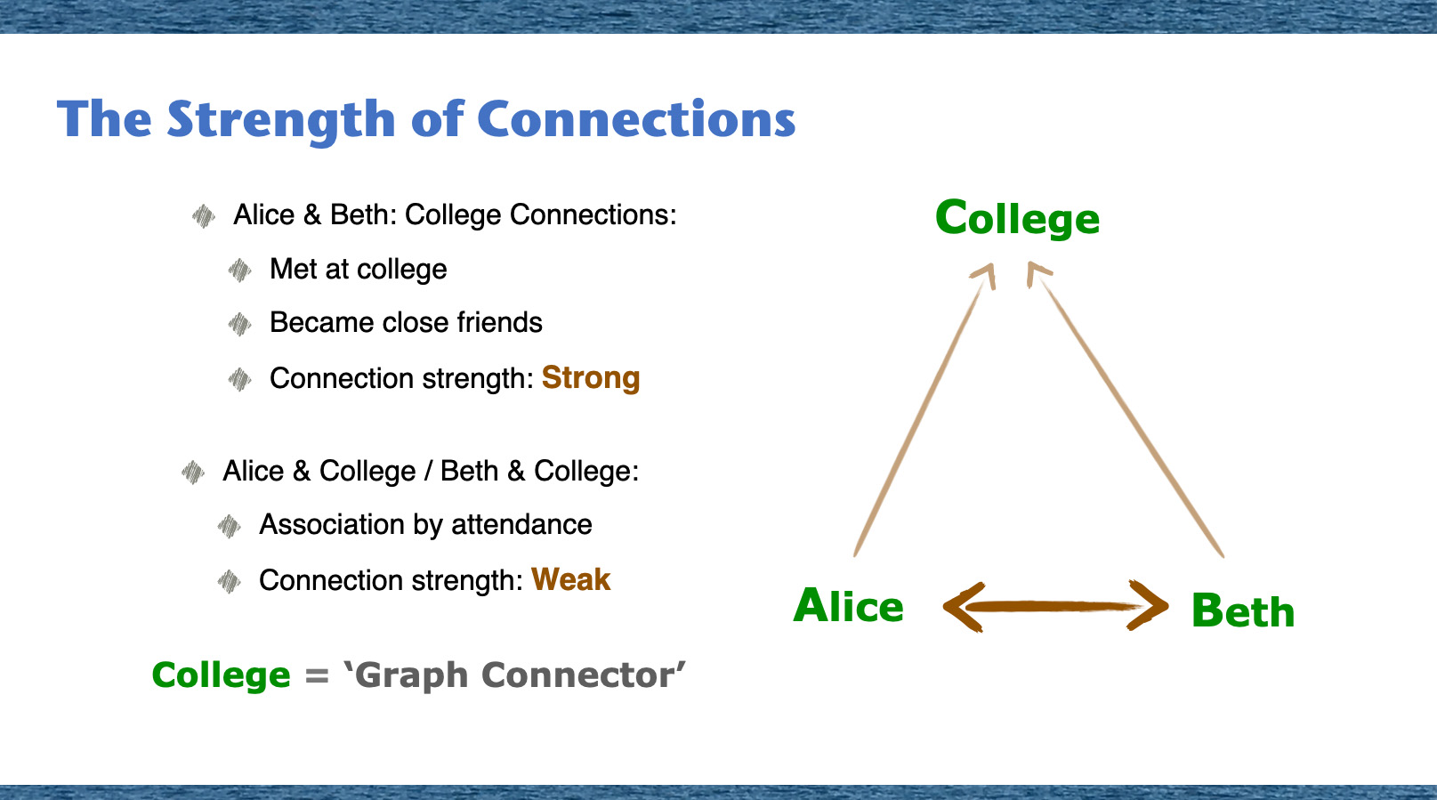
Analyzing graph triangles offers insights into the strength of connections between nodes within a network. Looking at the relationships among nodes A, B, and C, we are focusing on the strength of the connection between nodes A and B compared to the connections involving node C. Node C, identified as a 'graph connector' node, is critical in facilitating communication and interaction between nodes A and B. Serving as a link, node C allows the smooth flow of information and relationships between the strongly connected nodes A and B.
As analogy, imagine early 20th-century Vienna's intellectual scene as a dynamic network. Berta Zuckerkandl's salon stood out as one of central nodes, orchestrating and facilitating connections. Her salon served as the platform, connecting diverse talents like artists, scientists, and doctors. Each gathering at her salon can be seen as the creation of 'links' between nodes. Berta stands as a quintessential 'graph connector' and her role ensures not just random interactions, but impactful connections, emphasizing her integral position in this vibrant intellectual web.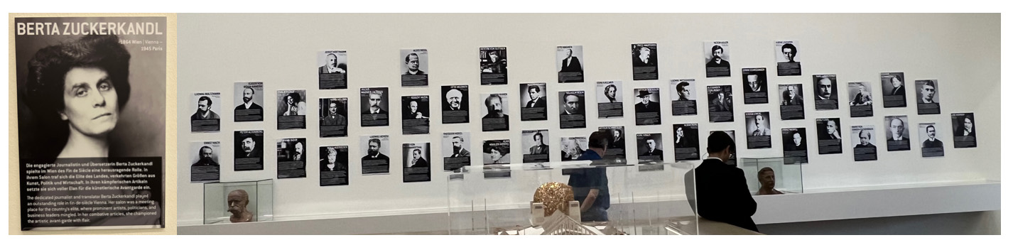 This characterizes the importance of graph connector nodes in enhancing the network's overall connectivity and functionality, fostering collective behaviors and dynamics among interconnected nodes.
Depicting Graph Connectors
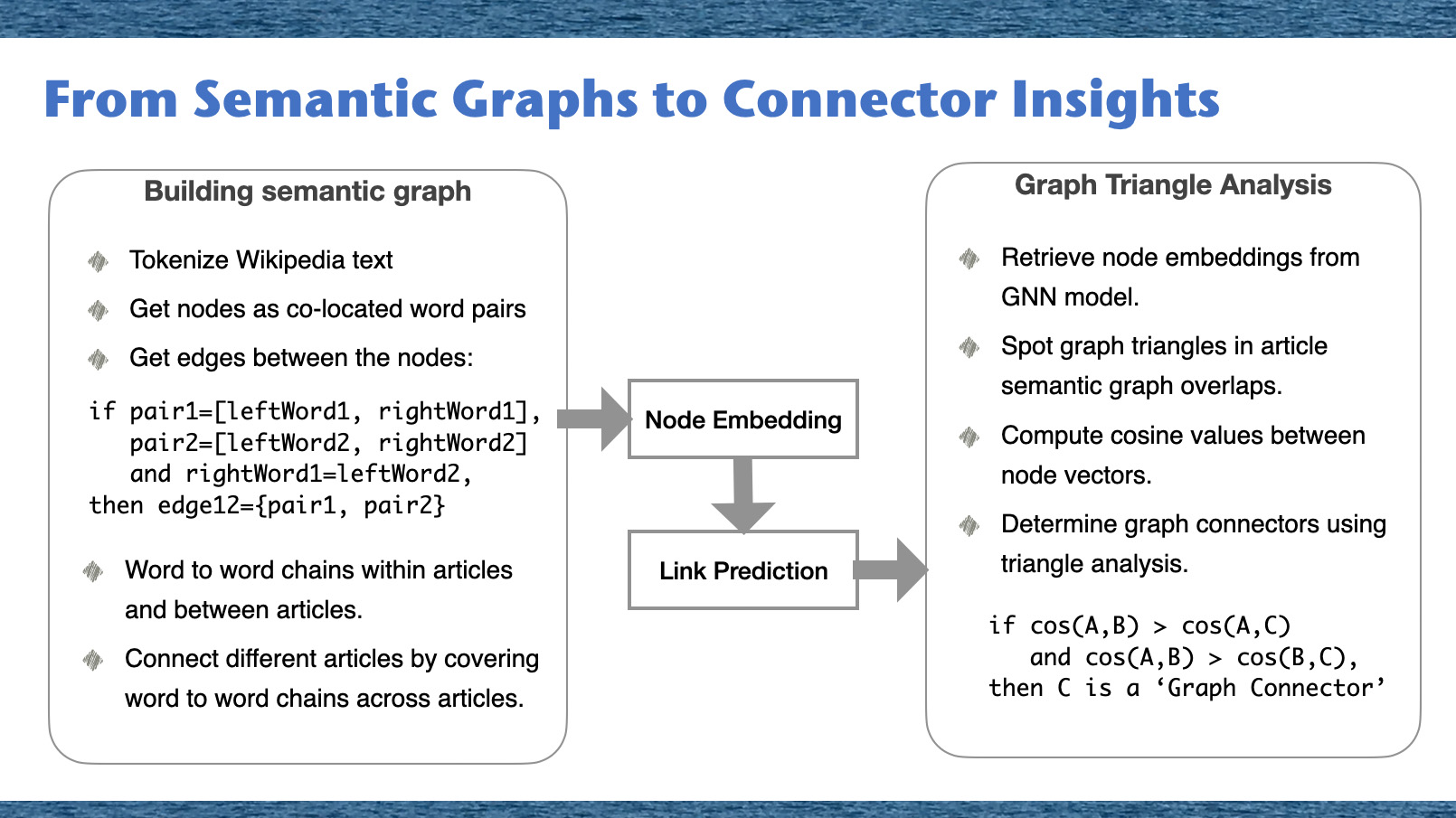
To find graph connectors, we will look for graph triangles where one cosine similarity between the nodes is higher than other two cosine similarity values. This implies a stronger connection between two nodes relative to the connections of two other node pairs. When delving into the world of graphs, it's essential to recognize the key players, the 'Graph Connectors'. These connectors serve as bridges within the intricate web of nodes. So, how do we uncover them? Let's take a journey through our method. First, we train our GNN Link Prediction model, which gives us the embeddings for each node. Think of these embeddings as unique signatures, encapsulating the essence of each node.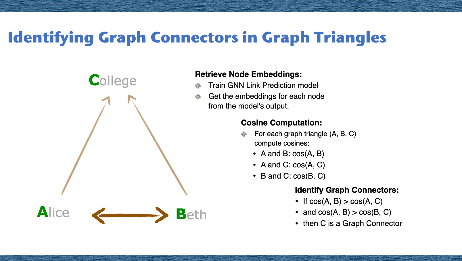 With these embeddings in hand, we compute the cosines between every pair of nodes in each graph triangle. These cosine values measure the similarity between nodes, indicating the strength of their connection.
Finally, the crux of our methodology: identifying the Graph Connectors. Based on our cosine computations, we determine which node acts as a bridge between the other two. For instance, in a triangle comprising nodes A, B, and C - if the connection strength between A and B surpasses the other two connections, it's clear that C plays the pivotal role of the connector.
This method thus allows us to highlight nodes that play an essential role in maintaining the structure and connectivity of the graph.
Graph representation traditionally operates in binary terms: either pairs of nodes are connected by edges or they are not. When using binary edges in graph triangle analysis, we are limited to recognizing the presence or absence of connections between nodes. Such a black-and-white perspective can overlook the nuanced graph connectors.
By employing GNN link prediction models, we move beyond this limitation. GNN link prediction model transcends this binary structure by embedding nodes into continuous vector space, providing a spectrum of ways to compare and evaluate these vectors. This deeper representation makes it possible to identify and understand graph connectors that a simple binary analysis might overlook.
In essence, understanding the nuances of node relationships allows for more robust, dynamic, and insightful analyses, enabling richer interpretations and predictions based on graph data.
With these embeddings in hand, we compute the cosines between every pair of nodes in each graph triangle. These cosine values measure the similarity between nodes, indicating the strength of their connection.
Finally, the crux of our methodology: identifying the Graph Connectors. Based on our cosine computations, we determine which node acts as a bridge between the other two. For instance, in a triangle comprising nodes A, B, and C - if the connection strength between A and B surpasses the other two connections, it's clear that C plays the pivotal role of the connector.
This method thus allows us to highlight nodes that play an essential role in maintaining the structure and connectivity of the graph.
Graph representation traditionally operates in binary terms: either pairs of nodes are connected by edges or they are not. When using binary edges in graph triangle analysis, we are limited to recognizing the presence or absence of connections between nodes. Such a black-and-white perspective can overlook the nuanced graph connectors.
By employing GNN link prediction models, we move beyond this limitation. GNN link prediction model transcends this binary structure by embedding nodes into continuous vector space, providing a spectrum of ways to compare and evaluate these vectors. This deeper representation makes it possible to identify and understand graph connectors that a simple binary analysis might overlook.
In essence, understanding the nuances of node relationships allows for more robust, dynamic, and insightful analyses, enabling richer interpretations and predictions based on graph data.
Employing Graph Triangle Analysis and the GraphSAGE Model
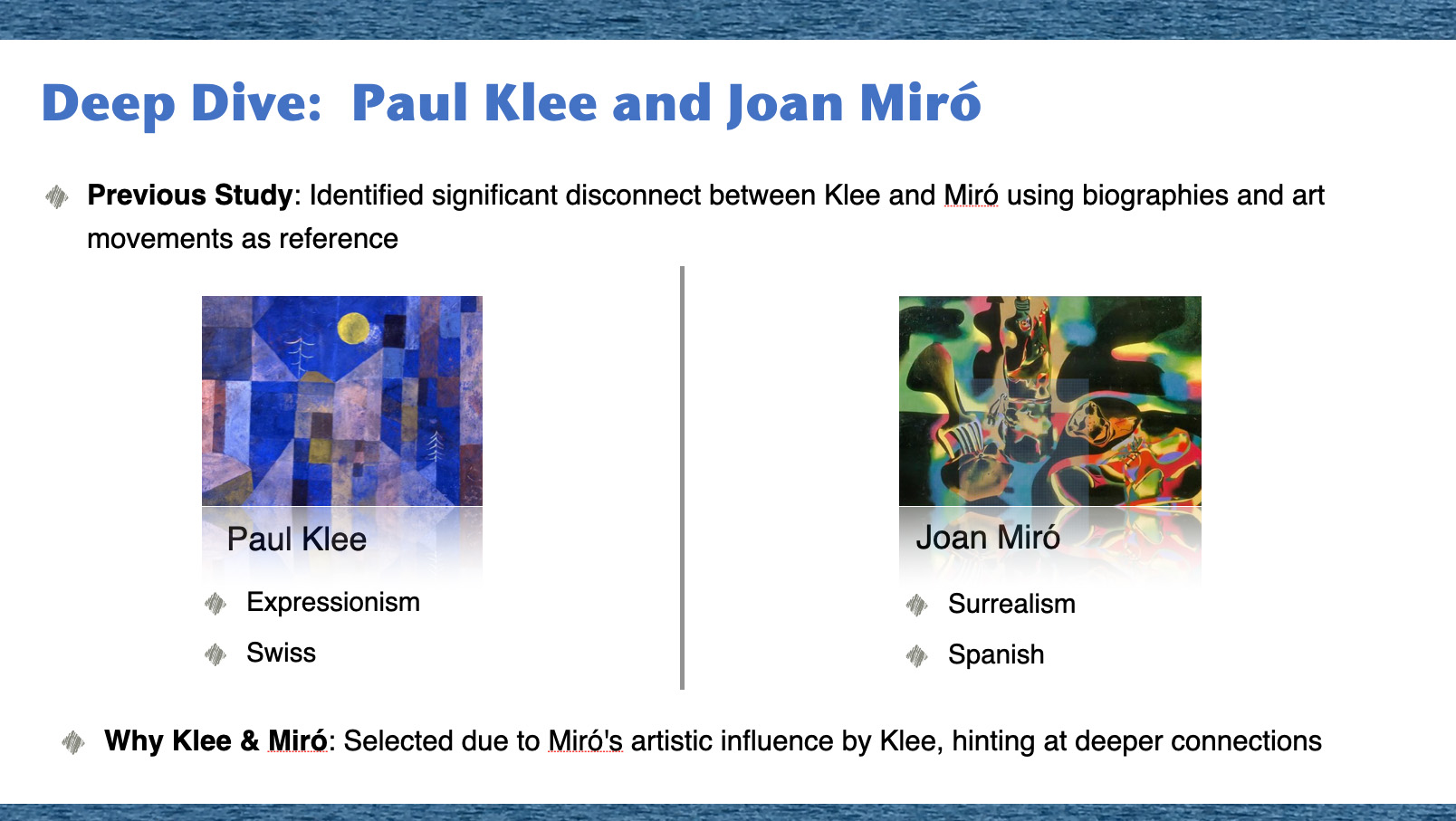
In this study, we aim to compare our previous study's results with the findings obtained through granular graph triangle analysis. Specifically, we'll examine the Wikipedia articles related to Paul Klee and Joan Miró, who were deemed as highly disconnected artists in the previous study. By employing graph triangle analysis techniques, we'll unveil previously overlooked graph connectors and patterns between these artists.
For our GNN link prediction model, we'll use the GraphSAGE model. Unlike traditional approaches relying on the entire adjacency matrix information, GraphSAGE focuses on learning aggregator functions. This allows us to generate embeddings for new nodes based on their features and neighborhood information without the need to retrain the entire model.
It's crucial to note that the outputs of the GraphSAGE model in our study are not actual predicted links, but embedded graphs. These embedded graphs capture the relationships and structural information within the original graphs. While these embeddings can be used for predicting graph edges, we will specifically utilize them for graph triangle analysis to identify and explore graph connectors within the network. These graph connectors play a pivotal role in facilitating connections and interactions between nodes, offering valuable insights into network dynamics and relationships.
Methods
Building a Knowledge Graph
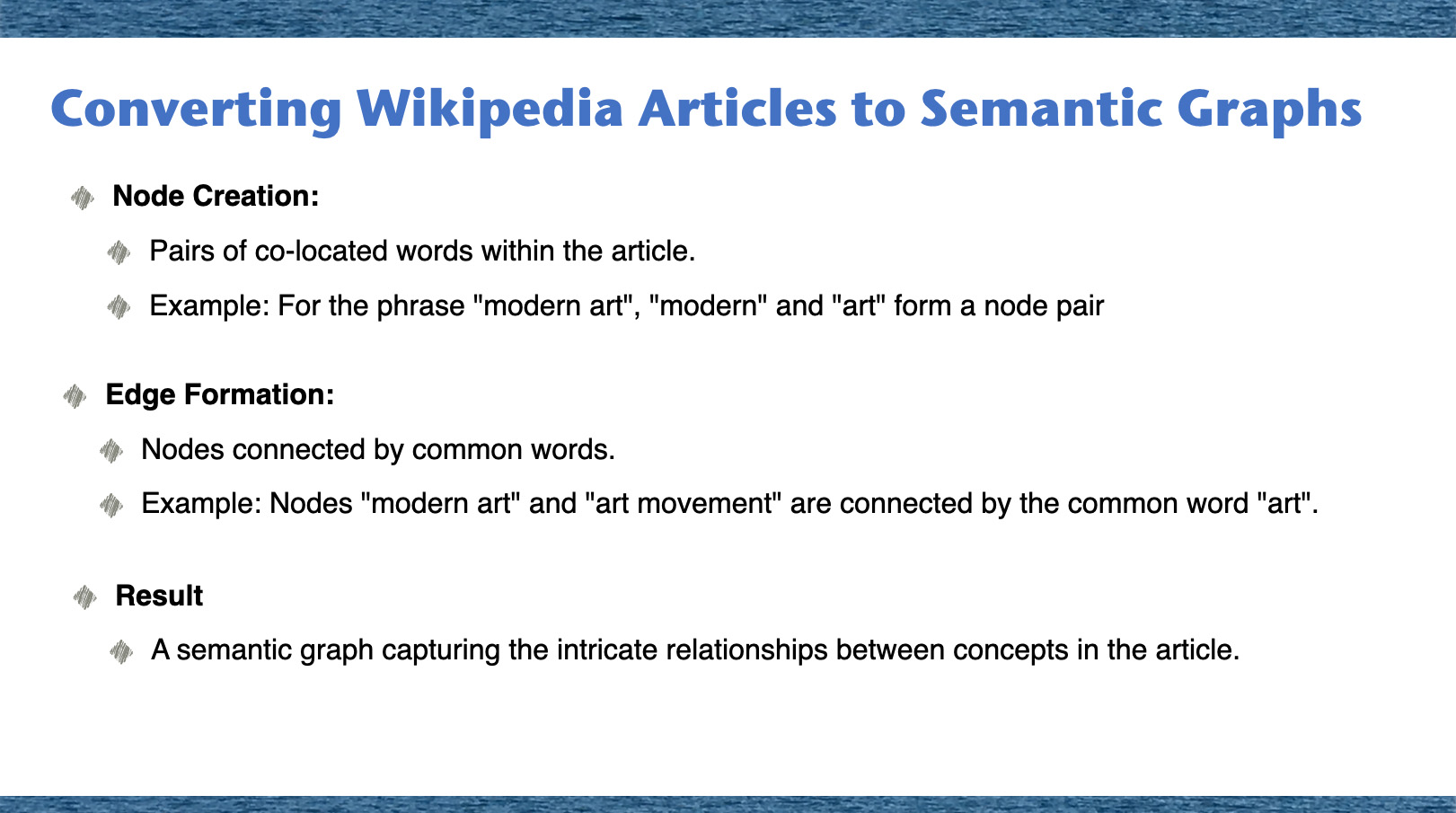
In this section, we'll outline our strategy to formulate an introductory knowledge graph for each article. Our approach uses co-located word pairs as nodes, establishing links between pairs sharing common words. The method can be detailed in the following steps:- Text Tokenization: Begin by breaking down the text from Wikipedia into individual words or 'tokens', while also excluding common stop words that don't contribute much to the overall meaning.
- Node Generation: Nodes in our knowledge graph are created from these co-located word pairs. These pairs of adjacent words from the text will form the basis of our graph.
- Edge Calculation: Edges are established between nodes that share common words. This generates a network of word chains within each article and enables the connection of different articles through these word chains. Conceptually, consider two pairs, pair1 and pair2, represented as:
    pair1=[leftWord1, rightWord1],
    pair2=[leftWord2, rightWord2]
edge12={pair1, pair2}
Node Embedding
To encapsulate the complexities of the knowledge graph into our nodes and translate the text information into vectors, we're utilizing the 'all-MiniLM-L6-v2' transformer model from Hugging Face. This model is a part of the sentence-transformers family, purposely built to convert text into a dense vector space. The resultant vector space has 384 dimensions, providing a rich and multidimensional representation of our textual information.Training a GNN Link Prediction Model
In our research, we've chosen to implement the GraphSAGE link prediction model proposed by Hamilton and others. This model is operationalized using the code provided in the DGL (Deep Graph Library) tutorial. It necessitates the transformation of the input graph data into an appropriate DGL data format. This transformation is a crucial step in preparing the data for the model training process.Triangle Analysis on Graphs
To delve deeper into the intricacies of graph structures, we used graph triangle analysis. Here's a step-by-step breakdown of our methodology:
- First, potential triangles are generated by considering all possible combinations of three distinct nodes from within the graph.
- Second, for each identified triangle, we compute the cosine similarities between the nodes. This involves calculating three cosine similarity values for each triangle - one for each pairing of nodes.
- Triangles of interest are those where one cosine similarity stands out as being notably higher compared to the other two values. This implies a stronger connection between two nodes relative to the connections of the other node pairs.
By focusing on such triangles, we can derive more insight into the underlying relationships between nodes. This allows us to uncover intricate patterns and gain a deeper understanding of the structural nuances present within the graph.
Experiments
In our exploration, we embarked on a transformative journey. We began by constructing semantic graphs, a process much like piecing together a puzzle, where each word forms a crucial piece, connecting with others to build a comprehensive picture. However, merely building the graph wasn't our end goal. To delve deeper into its intricate maze, we utilized Graph Triangle Analysis. This methodology allowed us to zoom in on specific relationships, akin to highlighting crucial intersections in a vast city map. It's through this refined lens that we transitioned from a broad understanding of the semantic landscape to pinpointing the connectors - the linchpins that hold the entire framework together, revealing a richer, more connected narrative.Data Source
As the data source for this study we used a subset of text data from Wikipedia articles about 20 modern art artists: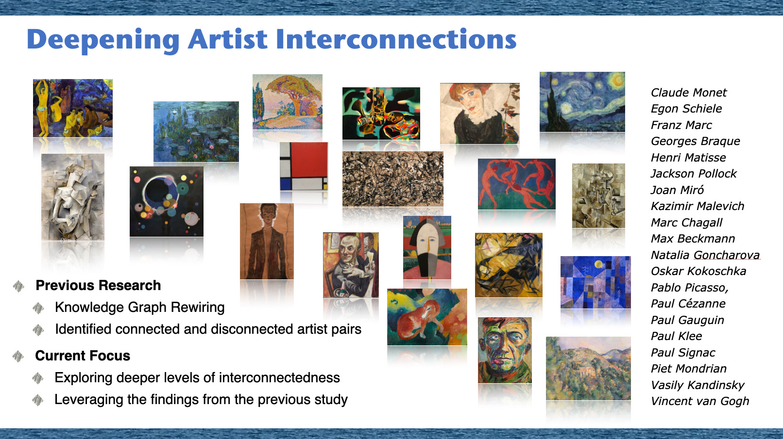 Building on our previous 'Knowledge Graph Rewiring' research, we initially identified artist connections. Now, we're digging deeper to uncover more intricate relationships between artists, using our past findings as a starting point.
In our pursuit of understanding artist interconnections, we took a focused look at two iconic figures of the art world: Paul Klee and Joan Miró. In our previous research, a curious observation emerged. Despite both artists being immersed in significant art movements, our data showed a pronounced disconnect between them. Klee, a Swiss maestro, was deeply rooted in Expressionism, while Miró, the Spanish virtuoso, was an embodiment of Surrealism. On the surface, these movements and their geographic roots seem to keep them apart. Yet, why did we zero in on these two? The intrigue lies in an understated influence: Miró's artistry was, in fact, inspired by Klee. This revelation hints at more profound, nuanced connections between them, suggesting that artistic interplay goes beyond just the obvious associations.
Building on our previous 'Knowledge Graph Rewiring' research, we initially identified artist connections. Now, we're digging deeper to uncover more intricate relationships between artists, using our past findings as a starting point.
In our pursuit of understanding artist interconnections, we took a focused look at two iconic figures of the art world: Paul Klee and Joan Miró. In our previous research, a curious observation emerged. Despite both artists being immersed in significant art movements, our data showed a pronounced disconnect between them. Klee, a Swiss maestro, was deeply rooted in Expressionism, while Miró, the Spanish virtuoso, was an embodiment of Surrealism. On the surface, these movements and their geographic roots seem to keep them apart. Yet, why did we zero in on these two? The intrigue lies in an understated influence: Miró's artistry was, in fact, inspired by Klee. This revelation hints at more profound, nuanced connections between them, suggesting that artistic interplay goes beyond just the obvious associations.
Preparation of Input Data
We constructed a knowledge graph based on co-located word pairs as described in the Methods. section. For model input data for this study we selected Wikipedia articles about Paul Klee and Joan Miró:
subsetWordpair = cleanPairWords.loc[:, ['idxArtist','wordpair','word1',	'word2'	]]
subsetWordpair = subsetWordpair[subsetWordpair['idxArtist'].isin([13,19])]
subsetWordpair.reset_index(inplace=True, drop=True)
nodeList=subsetWordpair
nodeList['idxPair'] = nodeList.index
Node list:
nodeList1=nodeList.rename({'word2':'theWord','wordpair':'wordpair1','wordPairIdx':'wordPairIdx1','idxArtist':'idxArtist1','idxPair':'idxPair1'}, axis=1)
nodeList2=nodeList.rename({'word1':'theWord','wordpair':'wordpair2','wordPairIdx':'wordPairIdx2','idxArtist':'idxArtist2','idxPair':'idxPair2'}, axis=1)
allNodes=pd.merge(nodeList1,nodeList2,on=['theWord'], how='inner')
Get unique word pairs for embedding:
bagOfPairWords=nodeList
bagOfPairWords.reset_index(inplace=True, drop=True)
bagOfPairWords['bagPairWordsIdx']=bagOfPairWords.index
Node embedding:
wordpair_embeddings = modelST.encode(bagOfPairWords["wordpair"],convert_to_tensor=True)
imgPath='/content/drive/My Drive/NLP/'
with open(imgPath+'wordpairs13b.pkl', "wb") as fOut:
    pickle.dump({'idx': bagOfPairWords["bagPairWordsIdx"],
                 'words': bagOfPairWords["wordpair"],
                 'artist': bagOfPairWords["idxArtist"],
                 'embeddings': wordpair_embeddings.cpu()}, fOut, protocol=pickle.HIGHEST_PROTOCOL)
Transform Data to DGL Format
We trained our GNN link prediction model using the GraphSAGE model from the DGL library. More in-depth information and coding techniques for data preparation and encoding data into the DGL data format are available in our post 'Find Semantic Similarities by GNN Link Predictions'. Import DGL andd read saved data:import dgl
import torch
import torch.nn as nn
import torch.nn.functional as F
import itertools
import numpy as np
import scipy.sparse as sp
import dgl.data
from dgl.data import DGLDataset
import os
with open(imgPath+'wordpairs13b.pkl', "rb") as fIn:
stored_data = pickle.load(fIn)
gnn_index = stored_data['idx']
gnn_artist = stored_data['artist']
gnn_words = stored_data['words']
gnn_embeddings = stored_data['embeddings']
df_gnn_words=pd.DataFrame(gnn_words)
df_gnn_words['idxNode']=df_gnn_words.index
Transform data to DGL format:
art_edges=allNodes[['idxPair1','idxPair2']]
unpickEdges=art_edges
edge_index=torch.tensor(unpickEdges[['idxPair1','idxPair2']].T.values)
u,v=edge_index[0],edge_index[1]
gNew=dgl.graph((u,v))
gNew.ndata['feat']=gnn_embeddings
gNew=dgl.add_self_loop(gNew)
g=gNew
Model Training
Split edge set for training and testingu, v = g.edges()
eids = np.arange(g.number_of_edges())
eids = np.random.permutation(eids)
test_size = int(len(eids) * 0.1)
train_size = g.number_of_edges() - test_size
test_pos_u, test_pos_v = u[eids[:test_size]], v[eids[:test_size]]
train_pos_u, train_pos_v = u[eids[test_size:]], v[eids[test_size:]]adj = sp.coo_matrix((np.ones(len(u)), (u.numpy(), v.numpy())))
adj_neg = 1 - adj.todense() - np.eye(g.number_of_nodes())
neg_u, neg_v = np.where(adj_neg != 0)
neg_eids = np.random.choice(len(neg_u), g.number_of_edges())
test_neg_u, test_neg_v = neg_u[neg_eids[:test_size]], neg_v[neg_eids[:test_size]]
train_neg_u, train_neg_v = neg_u[neg_eids[test_size:]], neg_v[neg_eids[test_size:]]
train_g = dgl.remove_edges(g, eids[:test_size])
from dgl.nn import SAGEConvclass GraphSAGE(nn.Module):
def __init__(self, in_feats, h_feats):
super(GraphSAGE, self).__init__()
self.conv1 = SAGEConv(in_feats, h_feats, 'mean')
self.conv2 = SAGEConv(h_feats, h_feats, 'mean')
def forward(self, g, in_feat):
h = self.conv1(g, in_feat)
h = F.relu(h)
h = self.conv2(g, h)
return h
train_pos_g = dgl.graph((train_pos_u, train_pos_v), num_nodes=g.number_of_nodes())
train_neg_g = dgl.graph((train_neg_u, train_neg_v), num_nodes=g.number_of_nodes())
test_pos_g = dgl.graph((test_pos_u, test_pos_v), num_nodes=g.number_of_nodes())
test_neg_g = dgl.graph((test_neg_u, test_neg_v), num_nodes=g.number_of_nodes())
import dgl.function as fn
class DotPredictor(nn.Module):
def forward(self, g, h):
with g.local_scope():
g.ndata['h'] = h
# Compute a new edge feature named 'score' by a dot-product between the
# source node feature 'h' and destination node feature 'h'.
g.apply_edges(fn.u_dot_v('h', 'h', 'score'))
# u_dot_v returns a 1-element vector for each edge so you need to squeeze it.
return g.edata['score'][:, 0]
class MLPPredictor(nn.Module):
def __init__(self, h_feats):
super().__init__()
self.W1 = nn.Linear(h_feats * 2, h_feats)
self.W2 = nn.Linear(h_feats, 1)
def apply_edges(self, edges):
h = torch.cat([edges.src['h'], edges.dst['h']], 1)
return {'score': self.W2(F.relu(self.W1(h))).squeeze(1)}
def forward(self, g, h):
with g.local_scope():
g.ndata['h'] = h
g.apply_edges(self.apply_edges)
return g.edata['score']
model = GraphSAGE(train_g.ndata['feat'].shape[1], 64)
pred = DotPredictor()
def compute_loss(pos_score, neg_score):
scores = torch.cat([pos_score, neg_score])
labels = torch.cat([torch.ones(pos_score.shape[0]), torch.zeros(neg_score.shape[0])])
return F.binary_cross_entropy_with_logits(scores, labels)
def compute_auc(pos_score, neg_score):
scores = torch.cat([pos_score, neg_score]).numpy()
labels = torch.cat(
[torch.ones(pos_score.shape[0]), torch.zeros(neg_score.shape[0])]).numpy()
return roc_auc_score(labels, scores)optimizer = torch.optim.Adam(itertools.chain(model.parameters(), pred.parameters()), lr=0.01)all_logits = []
for e in range(200):
# forward
h = model(train_g, train_g.ndata['feat'])
pos_score = pred(train_pos_g, h)
neg_score = pred(train_neg_g, h)
loss = compute_loss(pos_score, neg_score)
# backward
optimizer.zero_grad()
loss.backward()
optimizer.step()
if e % 5 == 0:
print('In epoch {}, loss: {}'.format(e, loss))from sklearn.metrics import roc_auc_score
with torch.no_grad():
pos_score = pred(test_pos_g, h)
neg_score = pred(test_neg_g, h)
print('AUC', compute_auc(pos_score, neg_score))- Number of nodes: 3,274
- Number of edges: 13,709
Interpret Model Results
Model results:gnnResults=pd.DataFrame(h.detach().numpy())import pandas as pd
from math import sin, cos, sqrt, atan2, radians
import torch
def pytorch_cos_sim(a: torch.Tensor, b: torch.Tensor):
return cos_sim(a, b)
def cos_sim(a: torch.Tensor, b: torch.Tensor):
if not isinstance(a, torch.Tensor):
a = torch.tensor(a)
if not isinstance(b, torch.Tensor):
b = torch.tensor(b)
if len(a.shape) == 1:
a = a.unsqueeze(0)
if len(b.shape) == 1:
b = b.unsqueeze(0)
a_norm = torch.nn.functional.normalize(a, p=2, dim=1)
b_norm = torch.nn.functional.normalize(b, p=2, dim=1)
return torch.mm(a_norm, b_norm.transpose(0, 1))cosine_scores_gnn = pytorch_cos_sim(h, h)Graph Triangle Analysis
Define graph and graph triangles:import networkx as nx
G=nx.from_pandas_edgelist(allNodes, "wordpair1", "wordpair2")
triangles = [clique for clique in nx.enumerate_all_cliques(G) if len(clique) == 3]triangleStats=[]
for triangle in triangles:
idx3=list(nodeList[nodeList['wordpair'].isin(triangle)]['bagPairWordsIdx'])
for pair1 in idx3:
for pair2 in idx3:
if (pair1<pair2):
score=dfWordPairs[(dfWordPairs['idx1']==pair1) & (dfWordPairs['idx2']==pair2)]['score'].values
triangleStats.append({'triangle':triangle,'pair1':pair1,'pair2':pair2,'score':score})triangleStatsDF=pd.DataFrame(triangleStats)
triangleStatsDF.to_csv(imgPath+'triangleStats.csv', index=False)Insights from Graph Triangles
In our exploration of the embedded graph triangles, we utilized ordered edge weights as a basis for analysis. From this process, we identified a total of 46 graph triangles. Among these, several met the criteria for containing a graph connector node, acting as a bridge or link between the other nodes within the graph triangle.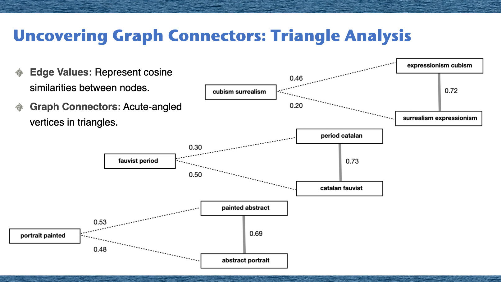 Our graph triangle analysis is illustrated in the fugure above. In this figure, the numbers you see next to each edge represent the cosine similarities between the vectors of the corresponding nodes. These numbers essentially reflect the strength of the connection between two nodes.
Imagine a vast network, a spider web of connections. Within this web, our goal was to uncover specific points, the linchpins holding everything together. These are our Graph Connectors. How do we identify them? We delve into Triangle Analysis. In this analysis, the sides of the triangles, the 'edges', represent how similar two nodes are to each other, quantified using cosine similarities. The Graph Connectors stand out as the acute-angled vertices, the points where threads converge sharply, indicating their pivotal role in the network's architecture. It's akin to finding the central anchors in our intricate web.
The patterns observed in these graph triangles provide valuable insights into the intricate relationships within our knowledge graph. More importantly, they shed light on the crucial role of graph connectors - the nodes that act as bridges, facilitating communication and interaction between other nodes within the graph triangle.
Our graph triangle analysis is illustrated in the fugure above. In this figure, the numbers you see next to each edge represent the cosine similarities between the vectors of the corresponding nodes. These numbers essentially reflect the strength of the connection between two nodes.
Imagine a vast network, a spider web of connections. Within this web, our goal was to uncover specific points, the linchpins holding everything together. These are our Graph Connectors. How do we identify them? We delve into Triangle Analysis. In this analysis, the sides of the triangles, the 'edges', represent how similar two nodes are to each other, quantified using cosine similarities. The Graph Connectors stand out as the acute-angled vertices, the points where threads converge sharply, indicating their pivotal role in the network's architecture. It's akin to finding the central anchors in our intricate web.
The patterns observed in these graph triangles provide valuable insights into the intricate relationships within our knowledge graph. More importantly, they shed light on the crucial role of graph connectors - the nodes that act as bridges, facilitating communication and interaction between other nodes within the graph triangle.
Observations and Insights
As we compare the results of our previous study 'Rewiring Knowledge Graphs by Link Predictions' with the findings of this current study, we can notice both similarities and differences in the outcomes.Similarities:
- Both studies utilized Wikipedia articles focusing on the biographies of modern art artists.
- The same semantic knowledge graph building method was employed in both studies.
- The GraphSAGE GNN link prediction model was utilized for graph embedding in both studies.
Differences:
- In the previous study, the GNN link prediction model results were aggregated by artists. The analysis suggested that Paul Klee and Joan Miró were highly disconnected artists.
- In contrast, the current study adopts a more granular approach to analyze the relationships between the artists. By using graph triangle analysis techniques, we were able to uncover potentially interesting relationships that were not previously identified.
The example graph triangles, like those seen in picture above, demonstrate the crucial role of graph connectors. The numbers placed next to the edges represent the cosine similarities between the vectors of the corresponding nodes, providing valuable insights into the relationships and patterns within the knowledge graph.
Conclusion
In this study, we utilized GNN link prediction techniques and graph triangle analysis to delve deeper into the intricacies of relationships within knowledge graphs. Leveraging these techniques, we demonstrated their potency in revealing patterns that might have previously gone unnoticed.
Our comparison between granular relationship analysis and aggregated relationships unveiled some compelling insights. In our previous study, based on an aggregated view, the artists Paul Klee and Joan Miró were deemed highly disconnected. However, that analysis failed to capture the finer nuances of their relationships. By applying graph triangle analysis techniques in this study, we found potentially significant connections and patterns between these artists, overlooked in the aggregated results.
This demonstrates the significance of granular analysis in comprehending the complex relationships within knowledge graphs. A deeper probe into the relationships between entities uncovers hidden associations and provides fresh insights into the interconnected data.
We have taken a step in exploring the concept of knowledge graph connectors. Through the use of GNN link prediction models and graph triangle analysis techniques, we have exposed the presence of graph connectors. These connectors play a critical role in facilitating connections and interactions between entities within the knowledge graphs.
Our study reveals new ways to understand complex connections in knowledge graphs, shedding light on hidden relationships and dynamics. This study is the beginning of a journey towards gaining a deeper understanding of the hidden relationships and dynamics within knowledge graphs.
Exploring Future Horizons with Graph Connectors
Envision the transformative impact of applying our advanced graph connector techniques across various fields:
- Medicine: Illuminate critical genetic pathways influencing diseases, paving the way for bespoke therapies and preventive measures.
- Social Networks: Uncover hidden influencers and emergent trends, reshaping our understanding of digital interactions.
- Finance: Identify key firms integral to market stability, potentially revolutionizing investment and economic strategies.
- Criminal Networks: Reveal the masterminds behind criminal activities, enhancing law enforcement capabilities.
- Education: Discover central interdisciplinary subjects that serve as educational connectors, promoting comprehensive learning experiences.
- Supply Chains: Spot critical intermediaries to streamline production, boosting efficiency and reducing operational costs.
The possibilities are boundless, and the diverse applications of our graph connector methods promise a future rich with insight and innovation!