Find Semantic Similarities by GNN Link Predictions

Link Prediction for Knowledge Graphs

In our previous post 'Rewiring Knowledge Graphs by Link Predictions' we showed how to rewire knowledge graph through GNN Link Prediction models. In this post we will continue discussion of applications of GNN Link Prediction techniques to rewiring knowledge graphs.

The goal of this post is the same as the goal of previous post: we want to find unknown relationships between modern art artists. We will continue exploring text data from Wikipedia articles about the same 20 modern art artists as we used in the previous post, but we will use a different approach to building initial knowledge graph: instead of building it on artist names and full text of corresponding Wikipedia articles we will build it on co-located word pairs.

Methods

Building initial Knowledge Graph

To build initial knowledge graph we will use the following steps:

• Tokenize Wikipedia text and exclude stop words.
• Get nodes as word pairs that are co-located within articles.
• Get edges as pair to pair neighbors following text sequences within articles.
• Get edges as joint pairs that have common words. These edges will represent word chains within articles and across them.

if pair1=[leftWord1, rightWord1],
   pair2=[leftWord2, rightWord2]
   and rightWord1=leftWord2,
then there is edge12={pair1, pair2}

Graph edges built based of these rules will cover word to word sequences and word to word chains within articles. More important, they will connect different articles by covering word to word chains across articles.

On nodes and edges described above we will built an initial knowledge graph.

Transform Text to Vectors

As a method of text to vector translation we will use 'all-MiniLM-L6-v2' transformer model from Hugging Face. This is a sentence-transformers model that maps text to a 384 dimensional vector space.

Run GNN Link Prediction Model

As Graph Neural Networks link prediction model we will use a GraphSAGE link prediction model from Deep Graph Library (DGL). The model is built on two GrapgSAGE layers and computes node representations by averaging neighbor information. The code for this model is provided by DGL tutorial DGL Link Prediction using Graph Neural Networks.

The results of this model are embedded nodes that can be used for further analysis such as node classification, k-means clustering, link prediction and so on. In this particular post we will calculate average vectors by artists and estimate link predictions by cosine similarities between them.

Cosine Similarities function:

import torch
def pytorch_cos_sim(a: Tensor, b: Tensor):
    return cos_sim(a, b)
def cos_sim(a: Tensor, b: Tensor):
    if not isinstance(a, torch.Tensor):
        a = torch.tensor(a)
    if not isinstance(b, torch.Tensor):
        b = torch.tensor(b)
    if len(a.shape) == 1:
        a = a.unsqueeze(0)
    if len(b.shape) == 1:
        b = b.unsqueeze(0)
    a_norm = torch.nn.functional.normalize(a, p=2, dim=1)
    b_norm = torch.nn.functional.normalize(b, p=2, dim=1)
    return torch.mm(a_norm, b_norm.transpose(0, 1))

Experiments

Data Source Analysis

As the data source for this study we used text data from Wikipedia articles about the same 20 artists that we used in our previous study "Building Knowledge Graph in Spark without SPARQL".

To estimate the size distribution of Wikipedia text data we tokenized the text and exploded the tokens:

from nltk.tokenize import RegexpTokenizer
tokenizer =RegexpTokenizer(r'[A-Za-z]+')

wikiArtWords=wikiArtists['Wiki']
  .apply(lambda x: RegexpTokenizer(r'[A-Za-z]+').tokenize(x)).reset_index()

wikiArtWords=wikiArtWords.explode(['words'])
wordStats=pd.merge(wikiArtWords,listArtists)

artistWordStats=wordStats.groupby('Artist').count()
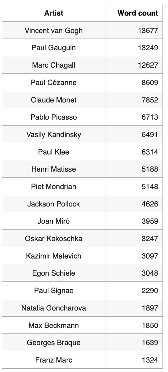
  .sort_values('words',ascending=False)

Based on Wikipedia text size distribution, the most well known artist in our artist list is Vincent van Gogh and the most unknown artist is Franz Marc:

Select Subsets of Words

Exclude stop words and short words woth length<4:

import nltk
nltk.download('stopwords')
from nltk.corpus import stopwords
STOPWORDS = set(stopwords.words('english'))
dfStopWords=pd.DataFrame (STOPWORDS, columns = ['words'])
dfStopWords['stop']="stopWord"
stopWords=pd.merge(wikiArtWords,dfStopWords,on=['words'], how='left')

nonStopWords=stopWords[stopWords['stop'].isna()]
nonStopWords['stop'] = nonStopWords['words'].str.len()
nonStopWords=nonStopWords[nonStopWords['stop']>3]
nonStopWords['words']= nonStopWords['words'].str.lower()
nonStopWords.reset_index(drop=True, inplace=True)
nonStopWords['idxWord'] = nonStopWords.index

The goal of this study is to find relationships between the artists. As Wikipedia articles about these artists have very different sizes, if we would use full Wikipedia text data, well-known artists who have longest articles would get more word pairs and much more connections than artists with shorter corresponding articles.

To balance artist to artist relationship distribution we selected subsets of articles with approximately the same word pair counts. As Wikipedia articles about artists all start with high level artist biography descriptions, from each article we selected the first 800 words.

nonStopWordsSubset = nonStopWords.groupby('idxArtist').head(800)
nonStopWordsSubset.reset_index(drop=True, inplace=True)
nonStopWordsSubset['idxWord'] = nonStopWordsSubset.index

Get Pairs of Co-located Words

Exclude stop words and short words woth length<4:

bagOfWords=pd.DataFrame(nonStopWordsSubset['words'])
bagOfWords.reset_index(drop=True, inplace=True)
bagOfWords['idxWord'] = bagOfWords.index

indexWords = pd.merge(nonStopWordsSubset,bagOfWords, on=['words','idxWord'])
idxWord1=indexWords
  .rename({'words':'word1','idxArtist':'idxArtist1','idxWord':'idxWord1'}, axis=1)
idxWord2=indexWords
  .rename({'words':'word2','idxArtist':'idxArtist2','idxWord':'idxWord2'}, axis=1)

leftWord=idxWord1.iloc[:-1,:]
leftWord.reset_index(inplace=True, drop=True)
rightWord = idxWord2.iloc[1: , :].reset_index(drop=True)  

pairWords=pd.concat([leftWord,rightWord],axis=1)
pairWords = pairWords.drop(pairWords[pairWords['idxArtist1']!=pairWords['idxArtist2']].index)
pairWords.reset_index(drop=True, inplace=True)

Drop duplicates {artist, word1, word2}

cleanPairWords = pairWords
cleanPairWords = cleanPairWords.drop_duplicates(
  subset = ['idxArtist1', 'word1', 'word2'], keep = 'last').reset_index(drop = True)
cleanPairWords['wordpair'] =
  cleanPairWords["word1"].astype(str) + " " + cleanPairWords["word2"].astype(str)
cleanPairWords['nodeIdx']=cleanPairWords.index
cleanPairWords.shape[0]
14933

Node examples:

nodeList=cleanPairWords
nodeList =nodeList.drop(['idxWord1','idxWord2','idxArtist2'], axis=1)
nodeList.head()
idxArtist1	word1	word2	wordpair	nodeIdx
0	0	braque	french	braque french	0
1	0	french	august	french august	1
2	0	august	major	august major	2
3	0	major	century	major century	3
4	0	century	french	century french	4

Get Edges

Index data:

nodeList1=nodeList
  .rename({'word2':'theWord','wordpair':'wordpair1','nodeIdx':'nodeIdx1'}, axis=1)
nodeList2=nodeList
  .rename({'word1':'theWord','idxArtist1':'idxArtist2','wordpair':'wordpair2',
  'nodeIdx':'nodeIdx2'}, axis=1)
allNodes=pd.merge(nodeList1,nodeList2,on=['theWord'], how='inner')
allNodes.shape
(231699, 2)

Save edges in Google Drive:

allNodes[['nodeIdx1','nodeIdx2']].to_csv(drivePath+"edges.csv", index=False)

Transform Text to Vectors

Transform node features to vectors and store in Google drive:

model = SentenceTransformer('all-MiniLM-L6-v2')
wordpair_embeddings = model.encode(cleanPairWords["wordpair"],convert_to_tensor=True)
wordpair_embeddings.shape
torch.Size([14933, 384])

Save nodes in Google Drive:

with open(imgPath+'wordpairs4.pkl', "wb") as fOut:
   pickle.dump({'idx': nodeList["nodeIdx"],
      'words': nodeList["wordpair"],
      'idxArtist': nodeList["idxArtist1"],
      'embeddings': wordpair_embeddings.cpu()}, fOut,
      protocol=pickle.HIGHEST_PROTOCOL)

Run GNN Link Prediction Model

As Graph Neural Networks (GNN) link prediction model we used a model from Deep Graph Library (DGL). The model code was provided by DGL tutorial and we only had to transform nodes and edges data from our data format to DGL data format.

Read embedded nodes and edges from Google Drive:

with open(drivePath+'wordpairs.pkl', "rb") as fIn:
    stored_data = pickle.load(fIn)
    gnn_index = stored_data['idx']
    gnn_words = stored_data['words']
    gnn_embeddings = stored_data['embeddings']

edges=pd.read_csv(drivePath + 'edges.csv')

Convert data to DGL format and add self-loop edges:

unpickEdges=edges
edge_index=torch.tensor(unpickEdges[['idx','idxNode']].T.values)
u,v=edge_index[0],edge_index[1]
g=dgl.graph((u,v))
g.ndata['feat']=gnn_embeddings
g=dgl.add_self_loop(g)

We used the model with the following parameters:

• 14933 nodes.
• 231699 edges.
• PyTorch tensor of size [14933, 384] for embedded nodes.

g
Graph(num_nodes=14933, num_edges=246632,
      ndata_schemes={'feat': Scheme(shape=(384,), dtype=torch.float32)}
      edata_schemes={})

For GraphSAGE model output vector size we experimented with sizes 32, 64 and 128:

model = GraphSAGE(train_g.ndata['feat'].shape[1], 128)

The model, loss function, and evaluation metric were defined the following way:

pred = DotPredictor()

def compute_loss(pos_score, neg_score):
    scores = torch.cat([pos_score, neg_score])
    labels = torch.cat([torch.ones(pos_score.shape[0]), torch.zeros(neg_score.shape[0])])
    return F.binary_cross_entropy_with_logits(scores, labels)

def compute_auc(pos_score, neg_score):
    scores = torch.cat([pos_score, neg_score]).numpy()
    labels = torch.cat(
        [torch.ones(pos_score.shape[0]), torch.zeros(neg_score.shape[0])]).numpy()
    return roc_auc_score(labels, scores)

To estimate the results we calculated accuracy metrics as Area Under Curve (AUC). For all three output vector sizes the model accuracy metrics were about 96 percents.

Rewiring Knowledge Graph by Predicted Links

The results of the GraphSAGE model from DGL library are not actually ‘predicted links’ but node vectors that were re-embedded by the model based on input node vectors and messages passed from the neighbors. They can be used for further analysis steps to predict graph edges.

The results of this scenario are 14933 reembedded nodes and to detect relationships between artists first, we calculated average node vectors by artists and then we estimated link predictions by cosine similarities between them.

As we mentioned above we experimented with GraphSAGE model output vector sizes of 32, 64 and 128 and compared distributions of cosine similarities between artist pairs.

First we looked at cosine similarity matrix for pairs of nodes embedded by GNN link prediction model:

cosine_scores_gnn = pytorch_cos_sim(h, h)

pairs_gnn = []
for i in range(len(cosine_scores_gnn)):
  for j in range(len(cosine_scores_gnn)):
    pairs_gnn.append({'idx1': i,'idx2': j,
      'score': cosine_scores_gnn[i][j].detach().numpy()})

    dfArtistPairs_gnn=pd.DataFrame(pairs_gnn)
    dfArtistPairs_gnn.shape
    (190, 3)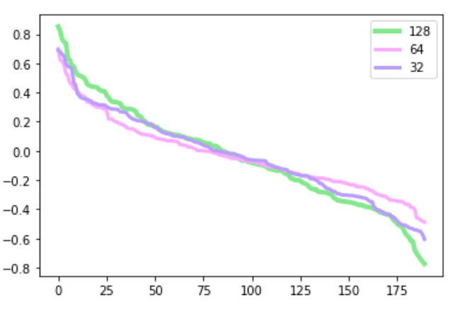

The number of cosine similarity pairs for 20 artists is 190 and the picture below illustrates cosine similarity distributions for model outputs of sizes 128, 64 and 32. For knowledge graph rewiring we selected the model results with output size 128 that reflects the most smooth cosine similarity distribution.

Results of Rewiring Knowledge Graph

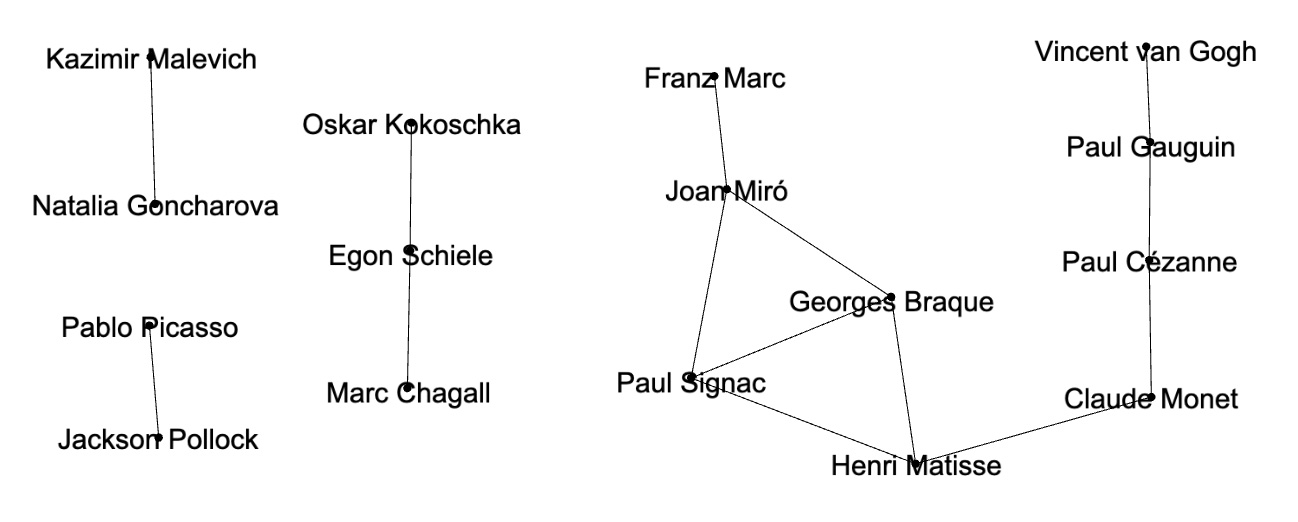
Artist pairs with cosine similarities > 0.5: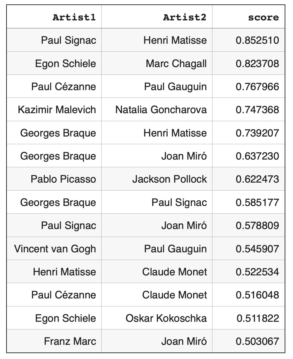

Graph illustration of artist pairs with hign cosine similarities > 0.5:

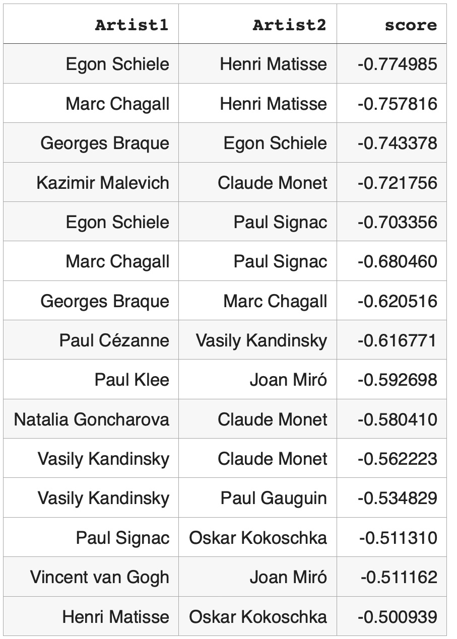
Pairs of artists with low cosine similarities < -0.5:

Observasions

Node pairs with high cosine similarities, also known as high weight edges, are actively used for graph mining techniques such as node classification, community detection or for analyzing node relationships.

In experiments of this study artist pairs with high cosine similarities can be considered as artist pairs with high semantic relationships through corresponding Wikipedia articles. Some of these relationships are well known: both Pablo Picasso and Georges Braque were pioneers of cubism art movement. Specialists in biographies of Paul Gauguin or Vincent van Gogh will not be surprised to find that these artists had high relationship regardless of their different art styles. Some undiscovered semantic connections such as between artists Egon Schiele and Marc Chagall might be interesting for modern art researchers.

Rewiring knowledge graph and finding high weight links between artists can be applied to recommender systems. If a customer is interested in Pablo Picasso art, it might be interesting for this customer to look at Georges Braque paintings or if a customer is interested in biography of Vincent van Gogh the recommender system can suggest to look at Paul Gauguin biography.

Applications of node pairs with high cosine similarities (or high weight edges) for graph mining techniques are well known: they are widely used for node classification, community detection and so on. On the other hand, node pairs with low cosine similarities (or negative weight edges) are not actively used. Based on our observations, dissimilar node pairs can be used for graph mining techniques in quite different way that similar node pairs or weakly connected node pairs.

For community detection validation strongly dissimilar node pairs act as more reliable indicators than weakly dissimilar node pairs: negative weight edges can validate that corresponding node pairs should belong to different communities.

Graphs with very dissimilar node pairs cover much bigger spaces that graphs with similar or weakly connected node pairs. For example, in this study we found low cosine similarities between key artists from not overlapping modern art movements: Futurism - Natalia Goncharova, Impressionism - Claude Monet and De Stijl - Piet Mondrian.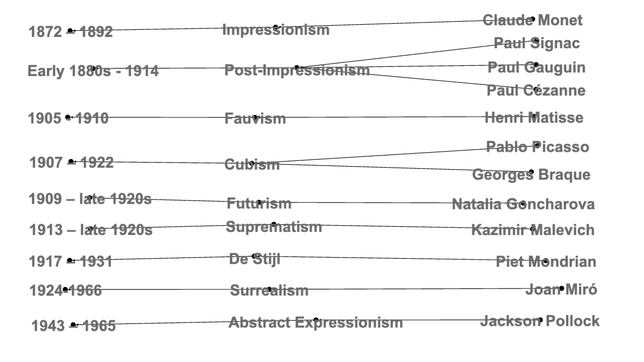

Links with very low cosine similarities can be used by recommender systems. If a customer is very familiar with Claude Monet’s style and is interested in learning about different modern art movements the recommender system might suggest to look at Piet Mondrian’s paintings or Natalia Goncharova’s paintings.

Conclusion

In this study we propose methods of rewiring knowledge graphs to detect hidden relationships between graph nodes by using GNN link prediction models.

In our experiments we looked at semantic similarities and dissimilarities between biographies of modern art artists by applying traditional and novel methods to their Wikipedia articles. Traditional method was implemented on full test of articles and cosine similarities between re-embedded nodes.

The novel method was based on distribution of co-located words within and across articles. The output vectors from GNN link prediction model were aggregated by artists and link predictions were estimated by cosine similarities between them.

We explored advantages for graph mining techniques of using not only highly connected node pairs but also highly disconnected node pairs. We denoted that level of disconnected word pairs can be used to define boundaries of a space covered by graph: existence of node pairs with very low cosine similarities shows that a graph covers much bigger space than a graph with only high and medium cosine similarities. Also highly disconnected node pairs are good indicators for validation of community detection.

We demonstrated applications of rewired knowledge graphs for recommender systems. Based on high similarity pairs recommender systems can suggest to look at paintings on biographies of artists that are similar to the artist of interest. Based on high dissimilarity pairs recommender systems can advice to look at very different art movements.

---

• ← Previous Post
• Next Post →