EEG Patterns by Deep Learning and Graph Mining

Bridges between AI and Neuroscience

Interactions between AI and cognitive science rapidly grow. By emulating how the brain acts, Artificial Intelligence became very successful in image recognition, language translation and many other areas. On the other hand, cognitive science is getting benefits from AI power as a model for developing and testing scientific hypothesis and studying patterns of neural activities recorded from the brain. How these two disciplines can help each other is well described by Neil Savage in the article "How AI and neuroscience drive each other forwards".

In this post we will analyze EEG data to distinguish between Alcoholic person behavior and behavior of person from Control group. To find behavior patterns in complex EEG signal data that consists from time series located on two-dimensional space we will:

Transform time series to images and use CNN image classifier methods
Transform time series to adjacency matrix for graph mining techniques

Why EEG Data?

EEG tools studying human behaviors are well described in Bryn Farnsworth's blog "EEG (Electroencephalography): The Complete Pocket Guide". There are several reasons why EEG is an exceptional tool for studying the neurocognitive processes:

EEG has very high time resolution and captures cognitive processes in the time frame in which cognition occurs.
EEG directly measures neural activity.
EEG is inexpensive, lightweight, and portable.
EEG data is publically available: we found this dataset in Kaggle.com

Machine Learning as EEG Analysis

Electroencephalography (EEG) is a complex signal and can require several years of training, as well as advanced signal processing and feature extraction methodologies to be correctly interpreted. Recently, deep learning (DL) has shown great promise in helping make sense of EEG signals due to its capacity to learn good feature representations from raw data. The meta-data analysis paper "Deep learning-based electroencephalography analysis: a systematic review" compares EEG deep learning with more traditional EEG processing approaches ans shows what deep learning approaches work and what do not work for EEG data analysis.

Our Method: CNN Classification of EEG Channel Time Series

In this post we will use another deep learning technique and make Time Series classification via CNN Deep Learning. We learned this technique in fast.ai 'Practical Deep Learning for Coders, v3' class and fast.ai forum 'Time series/ sequential data' study group.

We employed this technique for Natural Language Processing in our two previous posts - "Free Associations - Find Unexpected Word Pairs via Convolutional Neural Network" and "Word2Vec2Graph to Images to Deep Learning."

Our Method: Graph Community Detection

To find more explicit EEG channel patterns, we will use graph mining methods. We will transform EEG channel time series to vectors and build graphs on pairs of vectors with high cosine similarly. Using Graph connected components as community detection method will help us to find EEG channel time series patterns.

EEG Data Source

For this post we used EEG dataset that we found in kaggle.com website: 'EEG-Alcohol' Kaggle dataset. This dataset came from a large study of examining EEG correlates of genetic predisposition to alcoholism. We will classify EEG channel time series data to alcoholic and control person's EEG channels. Note: there are some data quality problems in this dataset.

Amount of subjects in each group is 8. The 64 electrodes were placed on subject's scalps to measure the electrical activity of the brain. The response values were sampled at 256 Hz (3.9-msec epoch) for 1 second. Each subject was exposed to either a single stimulus (S1) or to two stimuli (S1 and S2) which were pictures of objects chosen from the 1980 Snodgrass and Vanderwart picture set. When two stimuli were shown, they were presented in either a matched condition where S1 was identical to S2 or in a non-matched condition where S1 differed from S2.

EEG Channel CNN Classification

Classification Method

We will convert time series of EEG channels to images using Gramian Angular Field (GASF) - a polar coordinate transformation. This method is well described by Ignacio Oguiza in Fast.ai forum 'Time series classification: General Transfer Learning with Convolutional Neural Networks'. He referenced to paper Encoding Time Series as Images for Visual Inspection and Classification Using Tiled Convolutional Neural Networks. For data processing we will use ideas and code from Ignacio Oguiza code is in his GitHub notebook Time series - Olive oil country.

Transform Raw Data to EEG Channel Time Series (on Kaggle)

Kaggle EEG dataset was well analyzed in 'EEG Data Analysis: Alcoholic vs Control Groups' Kaggle notebook by Ruslan Klymentiev. We used his code for some parts of our data preparation. Here is raw data: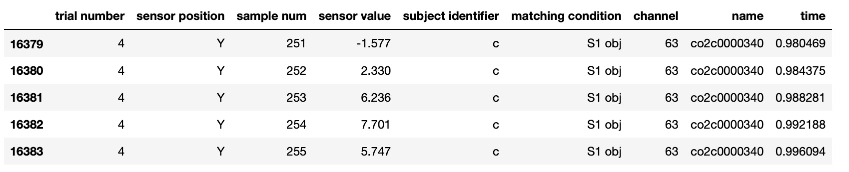

Python code to transform raw data to EEG channel time series data :

EEG_data['rn']=EEG_data.groupby(['sensor position','trial number',
   'subject identifier','matching condition','name']).cumcount()
EEG_TS=EEG_data.pivot_table(index=['trial number','sensor position',
    'subject identifier','matching condition','name','channel'],
    columns='rn',values='sensor value', aggfunc='first').reset_index()
EEG_TS.tail()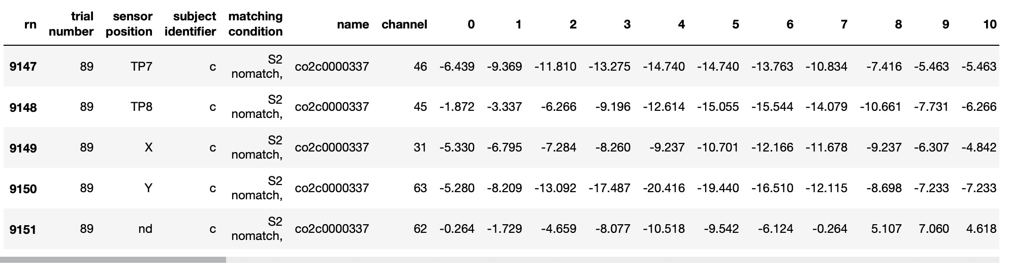

EEG channels - time series data:

Transform EEG Channel Time Series Data to Images (on Google Colab)

Python code to split data and transform time series to arrays:

import pandas as pd
a=pd.read_csv(filePath,sep=',',header=0).drop(a.columns[0], axis=1)
aa = a.reset_index(drop=True)
f=aa.iloc[:, [0,1,2,3,4,5 ]]
fx=aa.drop(aa.columns[[0,1,2,3,4,5]],axis=1).fillna(0).values

To convert time series to GASF images and classify images via CNN we used Python code that Ignacio Oguiza shared on fast.ai forum Time series - Olive oil country.

from pyts.image import GramianAngularField as GASF
image_size = 256
gasf = GASF(image_size)
fX_gasf = gasf.fit_transform(fX)
plt.figure(figsize=(8, 8))

EEG Channel Images - Examples

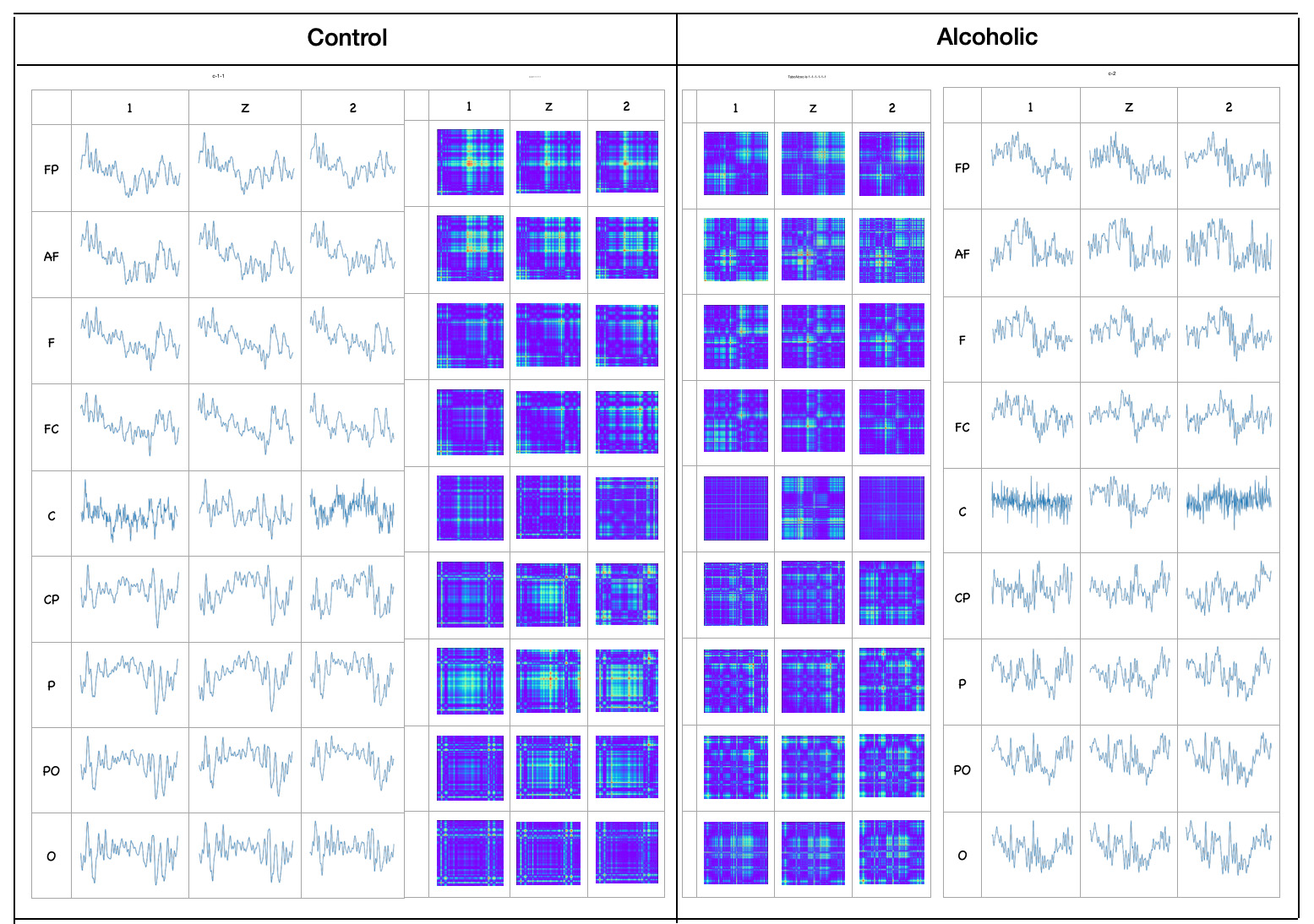
As image examples we will show line graph pictures and GASF images for EEG channels on F8 and T7 positions of one person from Alcoholic group and one person from Control group. All time series were taken from "two stimuli - match" trial.

idxList1=f.index[(f['sensor position'] == 'F8')&
   (f['matching condition'] == 'S2 match')&   
   (f['name']=='co2a0000365')].tolist()[0]
plt.plot(fX[idxList1])
plt.imshow(fX_gasf[idxList1], cmap='rainbow', origin='lower')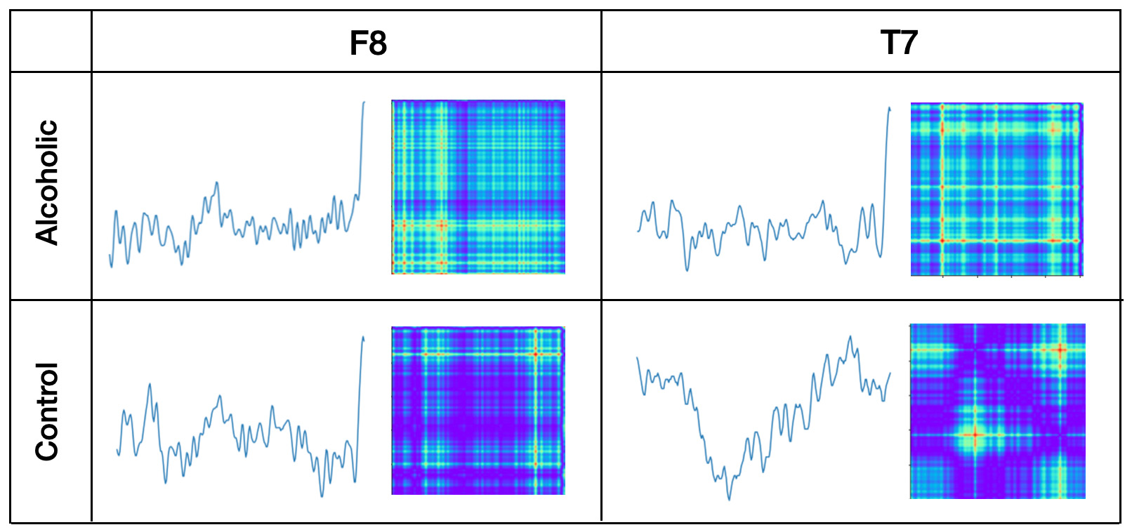

Observations:

Alcoholic person's F8 and T7 time series look closer than Control person's F8 and T7 time series
There are more differences between Alcoholic and Control person's time series than between F8 and T7 time series

Generate and Save Images

Generated images of EEG channel time series were stored in classification subdirectories:

numRows=f.shape[0]
for i in range(numRows):
    if not os.path.exists(IMG_PATH):
        os.makedirs(IMG_PATH)  
    idxPath = IMG_PATH +'/' + str(f['subject identifier'][i])
    if not os.path.exists(idxPath):
        os.makedirs(idxPath)
    imgId = (IMG_PATH +'/' +  
       str(f['subject identifier'][i])) +'/' +
       str(f['sensor position'][i]+'~'+
       str(f['channel'][i])+'~'+f['name'][i]+'~'+
       str(f['trial number'][i])+'~'+f['matching condition'][i])    
    plt.imshow(fX_gasf[i], cmap='rainbow', origin='lower')   
    plt.savefig(imgId, transparent=True)
    plt.close()

Image Classification

EEG channel time series classification was done on fast.ai transfer learning approach:

from fastai.text import *
from fastai.vision import learner
PATH_IMG=IMG_PATH
tfms = get_transforms(do_flip=False,max_rotate=0.0)
np.random.seed(42)
data = ImageDataBunch.from_folder(PATH_IMG,  train=".", valid_pct=0.21, size=256)
learn = learner.cnn_learner(data, models.resnet34, metrics=error_rate)
learn.fit_one_cycle(8)

EEG Channels Classification Metrics

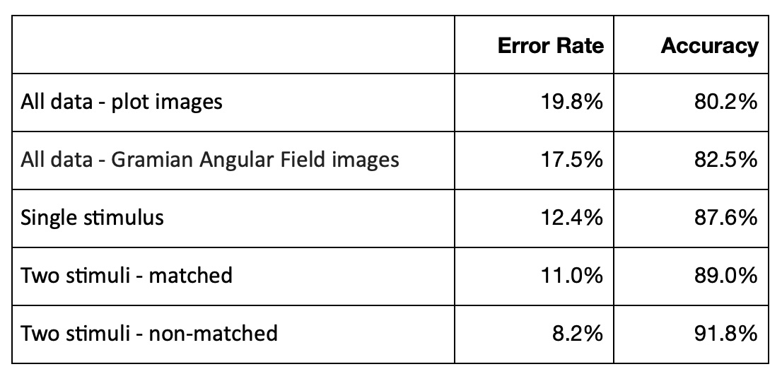
Here are cycle metrics for GASF image classification: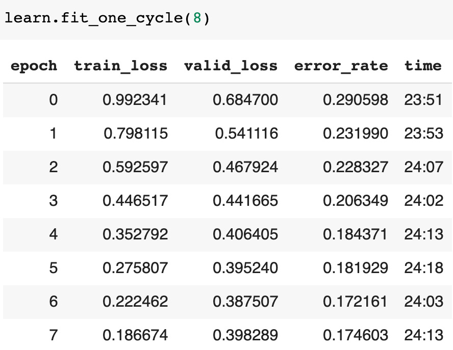

Tuning classification model we've got about 80.2% accuracy for graph line image classification and 82.5% accuracy for GASF image classification. Accuracy metrics for data separated by different types of stimulus are higher than for all data classifying together. The highest accuracy metric - 91.8% we've got for "two non-matched stimuli".

Graph Connections between EEG Channels

Building Graph in Spark (on Databricks)

We will build EEG channel graph in scala Spark using Spark GraphFrames library. We will build graphs and define EEG time series patterns on a subset of data: we will take one person from Alcoholic group and one person from Control group. For each person we will select three trials of different types.

Data Processing

As raw data we will use the same EEG channel time series data that we generated from Kaggle dataset and used for CNN image classification:

Data processing:

Read EEG_TS.csv file
Transform columns [0, 1, ..., 255] from strings to double.
Rename these columns as ['arr0', 'arr1', ..., 'arr255']
Extract from schema all columns with names like 'arr*'

import org.apache.spark.sql.functions.{col, lit, when}
import org.apache.spark.sql.functions._
import org.apache.spark.sql.expressions.Window
import org.graphframes._
import org.graphframes.examples

val dataInput=spark.read.option("header",true).csv("FileStore/tables/EEG_TS.csv")
val colList=dataInput.schema.fieldNames
var dataInputTable=dataInput.withColumn("arr0",lit("#"))
for(ind <- (0 to 255)){
   dataInputTable=dataInputTable.
     withColumn("arr"+lit(ind),col(ind.toString).cast("double"))
}
val arrColList=dataInputTable.schema.fieldNames.filter(s=>(s.contains("arr")))

Convert to vectors:

Transform collumns [arr0,...,arr255] to vectors.
Generate a table as a combination of paramaters "trial number", "sensor position", "subject identifier", "matching condition", "name", "channel" and vectors.

import org.apache.spark.mllib.linalg._
import org.apache.spark.mllib.linalg.Vector
import org.apache.spark.mllib.linalg.{Vectors, Vector}
import org.apache.spark.ml.feature.VectorAssembler

val assembler = new VectorAssembler().
setInputCols(arrColList).
setOutputCol("vector")
val output = assembler.transform(dataInputTable)
val dataVector=output.select("trial number", "sensor position",
   "subject identifier", "matching condition", "name", "channel","vector")
val dataVector=output.select("trial number", "sensor position",
   "subject identifier", "matching condition", "name", "channel","vector")

Select Data Subsets

We selected the following data subsets: one person from each group and one trial of each type.

one person from Alcoholic group: "co2a0000364"
one person from Control group:"co2c0000340"
"S1 obj": single stimulus
"S2 match": two stimuli - matched
"S2 nomatch": two stimuli - non-matched

val dataSampleC=dataVector.filter(col("name").isin("co2a0000364","co2c0000340")).
   filter(col("trial number").isin(2,25,14,31,75,83))
display(dataSampleC.groupBy("trial number",
   "matching condition","name").count.orderBy("name","matching condition"))
   trial number,matching condition,name,count
   2,S1 obj,co2a0000364,64
   25,S2 match,co2a0000364,64
   31,S2 nomatch,co2a0000364,64
   14,S1 obj,co2c0000340,64
   75,S2 match,co2c0000340,64
   83,S2 nomatch,co2c0000340,64

Build Graphs and Find Patterns

For each {person, trial} we will:

create adjacency matrix
calcultate cosine similarities between vectors
select pairs with cosines higher than threashold 0.9
build a graph
calcultate graph connected components

Self-join the vector table:

val dataVectorC1=dataSampleC.
   select("matching condition","subject identifier","name",
   "sensor position","channel","vector").
   toDF("condition1","flag1","name1","position1","channel1","vector1")
val dataVectorC2=dataVectorC1.
  toDF("condition2","flag2","name2","position2","channel2","vector2")
val dataVectorC12=dataVectorC1.
  join(dataVectorC2,'position1=!='position2  &&  'channel1=!='channel2)

Calcultate adjacency matrix:

def dotVector(vectorX: org.apache.spark.ml.linalg.Vector,
   vectorY: org.apache.spark.ml.linalg.Vector): Double = {
   var dot=0.0
   for (i <-0 to vectorX.size-1) dot += vectorX(i) * vectorY(i)
   dot
}
def cosineVector(vectorX: org.apache.spark.ml.linalg.Vector,
   vectorY: org.apache.spark.ml.linalg.Vector): Double = {
   require(vectorX.size == vectorY.size)
   val dot=dotVector(vectorX,vectorY)
   val div=dotVector(vectorX,vectorX) * dotVector(vectorY,vectorY)
   if (div==0)0
   else dot/math.sqrt(div)
}
val dataVectorCcosMatrix=dataVectorC12.
   map(r=>(r.getAs[String](0),r.getAs[String](1),r.getAs[String](2),
   r.getAs[String](3),r.getAs[String](4),r.getAs[String](6),
   r.getAs[String](7),r.getAs[String](8),r.getAs[String](9),
   r.getAs[String](10),cosineVector(r.getAs[org.apache.spark.ml.linalg.Vector](5),
   r.getAs[org.apache.spark.ml.linalg.Vector](11)))).
   toDF("condition1","flag1","name1","position1","channel1","condition2",
   "flag2","name2","position2","channel2","cos12")

Build a graph. Subset example: person name="co2a0000364" and condition="S2 match":

val graphEdges= dataVectorCcosMatrix.filter('condition1==='condition2).
   filter('name1==='name2).
   filter('cos12>0.9).
   filter('name1==="co2a0000364").
   filter('condition1==="S2 match").
   select("position1","position2","condition1").
   filter('position1<'position2).
   toDF("src","dst","edgeId").distinct
val graphNodes= graphEdges.select("src").
   union(graphEdges2.select("dst")).distinct.toDF("id")
val graph = GraphFrame(graphNodes,graphEdges)

Calcultate graph connected components and connected component size distribution:

val graphCC = graph.
     connectedComponents.run()
val graphCCcount=graphCC.
     groupBy("component").count.
     toDF("cc","ccCt")

Graph Visualization

For graph visualization we use Gephi tool. Gephi takes DOT graph language and allows to authomatically define node and edge colors.

Define nodes and edges colors:

display(dataCC.select("name","condition","component","id").orderBy("name","condition","component","id"))
name,condition,component,id
co2a0000364,S1 obj,103079215104,AF1
co2a0000364,S1 obj,103079215104,AF2
co2a0000364,S1 obj,103079215104,AF7
co2a0000364,S1 obj,103079215104,AF8
co2a0000364,S1 obj,103079215104,AFZ
co2a0000364,S1 obj,103079215104,F1
co2a0000364,S1 obj,103079215104,F2

To compare patterns within the same picture, we will define colors as different colors for different connected components within each graph as well as the same color for similar connected components of different graphs:

val dataColor=dataCC.
   withColumn("minW",min("id").over(Window.
     partitionBy("name","condition","component"))).       
   withColumn("rn",row_number.over(Window.
     partitionBy("name","condition","component").orderBy("id"))).
   withColumn("color",when(col("minW").rlike("AF"),lit("darkorange")).
   when(col("minW").isin("CP1","CP4","CZ"),lit("steelblue1")).
   when(col("minW").isin("CP6"),lit("azure4")).
     otherwise(lit("forestgreen")))
display(dataColor.select("name","condition", "component","minW","color").
   distinct.orderBy("name","condition","minW"))
name,condition,component,minW,color
co2a0000364,S1 obj,103079215104,AF1,darkorange
co2a0000364,S1 obj,412316860416,CP1,steelblue1
co2a0000364,S1 obj,51539607552,CP2,forestgreen
co2a0000364,S2 match,103079215104,AF1,darkorange
co2a0000364,S2 match,51539607552,CP1,steelblue1
co2a0000364,S2 nomatch,103079215104,AF2,darkorange
co2a0000364,S2 nomatch,51539607552,CP4,steelblue1
co2a0000364,S2 nomatch,644245094400,P1,forestgreen
co2c0000340,S1 obj,103079215104,AF1,darkorange
co2c0000340,S1 obj,558345748481,C5,forestgreen
co2c0000340,S1 obj,51539607552,CP1,steelblue1
co2c0000340,S2 match,103079215104,AF1,darkorange
co2c0000340,S2 match,25769803776,C6,forestgreen
co2c0000340,S2 match,1279900254208,CP6,azure4
co2c0000340,S2 match,51539607552,CZ,steelblue1
co2c0000340,S2 nomatch,25769803776,AF1,darkorange
co2c0000340,S2 nomatch,51539607552,CP1,steelblue1

Example: node colors for connected components of graph with name="co2a0000364" and condition="S2 match":

display(dataColor.filter('name==="co2a0000364").
   filter('condition==="S2 nomatch").select("id","color").
   distinct.toDF("colorId","color").   
   map(s=>("\""+s(0).toString +"\""+" [color="+s(1).toString +"];")).
   toDF("colorLine"))
colorLine
"AF7" [color=darkorange];
"AFZ" [color=darkorange];
"CP4" [color=steelblue1];
"F1" [color=darkorange];
"F2" [color=darkorange];
"P5" [color=forestgreen];
"P6" [color=steelblue1];
"P8" [color=steelblue1];

Transform graph edges to DOT language:

display(graph2.edges.map(s=>("\""+s(0).toString +"\" -- \""
   +s(1).toString +"\""+" [label=\""+s(2).toString+"\"];")).toDF("dotLine") )
dotLine
"P1" -- "POZ" [label="S2 match"];
"P2" -- "PO2" [label="S2 match"];
"F1" -- "FZ" [label="S2 match"];
"O2" -- "POZ" [label="S2 match"];
"AFZ" -- "F1" [label="S2 match"];
"F1" -- "F3" [label="S2 match"];
"AF1" -- "FZ" [label="S2 match"];
"AF7" -- "FP1" [label="S2 match"];
"OZ" -- "PO2" [label="S2 match"];
"O2" -- "PO1" [label="S2 match"];

EEG Channel Patterns

All graphs show that time series Two stimuli non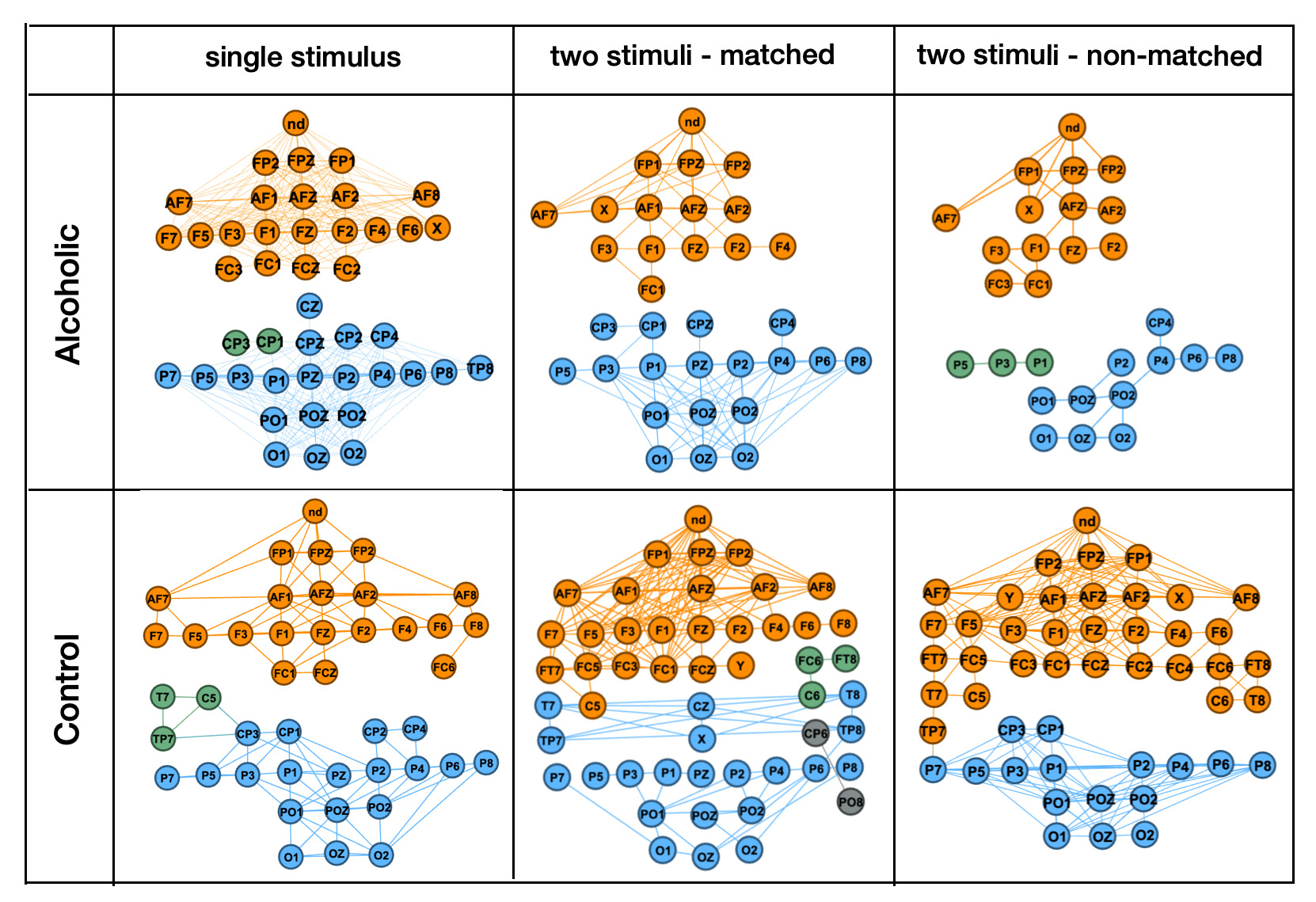

Observations:

All graphs have separate patters for front and back
"Single stimulus" patters are not very different between persons from Alcoholic and Control groups
The biggest difference between Alcoholic and Control person patters is in trial for "two stimuli, non-matched" patterns. This corresponds with image classifier metrics: "two stimuli, non-matched" trial has the highest accuracy in classifying alcoholic verses control group behaviors.
Control group person's patters for both "two stimuli" trials are much tighter connected then for person from Alcoholic group.

Here is another view: pictures of EEG channel time series for "two stimuli, non-matched" patterns for the same persons that we analyzed through graph mining. It presents images around 'Z' lines. This images show more details on EEG channel time series, not only the fact that pairs of vectors have high cosine similarities.

AI, Graphs and Neuroscience

Why Artificial Intelligence is behind of human brain? Stanislas Dehaene, psychologist and cognitive neuroscientist, in his book "How We Learn: Why Brains Learn Better Than Any Machine...for Now" argues that deep learning algorithms mimic only a small part of our brain’s functioning, the first two or three hundred milliseconds during which our brain operates in an unconscious manner. Only in the subsequent stages, which are much slower, more conscious, and more reflective, does our brain manage to deploy all its abilities of reasoning, inference, and flexibility—features that today’s machines are still far from matching.

Graph Brain Theory

In this post we indicated how graph mining methods can uncover hidden patters. Like human brains, graphs can connect the dots, perform cognitive inference, empower machines to detect hidden patterns, and most importantly, derive insights from the vast amount of heterogeneous data and play significant role in studying the human brain network - connectome.

More important, graph technology conforms with Konstantin Anokhin's Hypernetwork Brain Theory (HBT): "Cognitome: Neural Hypernetworks and Percolation Hypothesis of Consciousness" . This theory suggests that evolution, development and learning shape neural networks (connectome) into a higher-order structures - cognitive neural hypernetworks (cognitome).

Each brain at its maximal causal power is cognitome - a neural hypernetwork with emergent cognitive properties. Vertices of cognitome - GOgnitive Groups (COGs) - are subsets of elements from the underlying neuronal network that are associated by a common experience. Edges between COGs - Links Of Cogs (LOCs) - represent units of causal knowledge of a cognitive agent. HBT describes various mental processes as different forms of traffic in this hypernetwork.

Graph Tecnology Trends

Two trends of practical graph applications are following the brain - graph relationships: Property Graphs and Knowledge Graphs. Technically property graphs and knowledge graphs can be implemented by analogous techniques, conceptually these trends are quite different. Property graphs usualy considered from graph theory point of view representing networks of similar nodes like what we demonstrated in this post. Communitied within these graphs can be seen as COGs.

Knowledge graphs are like machine readable "grandmother cells": type "Eiffel Tower" and in Google Knowledge Graph you will see pictures, map, and text about Eiffel Tower as well as links to Paris, Louvre, and so on. If you hear or read the words "Eiffel Tower" you'll imaging it's pictures, think about Paris, and so on. Your COGs and LOCs, your thinking movement will be specific to your experience and depend on many things around you.

Graphs, AI and Neuroscience

Graph trends that are following the brain - graph relationships and act as cognitive inference, are based on traditional programming and far from using deep learning techniques. The reasons why graphs are not in AI yet is well described in Michael Bronstein's article "Do we need deep graph neural networks?"

In addition to general graph theory reasons, knowledge graphs are usualy built on conservative Semantic Web style, with SPARQL and OWL languages. This explains why knowledge graphs are only considered as complimentary tools for Artificial Intelligence: they are used either for data integration or for Explainable AI. Even in EU-funded Human Brain Project knowledge graph is only used as a metadata management system built for EBRAINS: "EBRAINS Knowledge Graph"

We hope that in the future, when deep learning techniques on graph technology will evolve, graphs will support AI ability for inference and reasoning.

Next Post - EEG analysis

In the next several posts we will continue building bridges between AI, graphs and neuroscience.