Unsupervised Deep Learning for Climate Data Analysis

Unsupervised CNN Deep Learning Classification

Outstanding success of Convolutional Neural Network image classification in the last few years influenced application of this technique to extensive variety of objects. CNN image classification methods are getting high accuracies but they are based on supervised machine learning, require labeling of input data and do not help to understand unknown data.

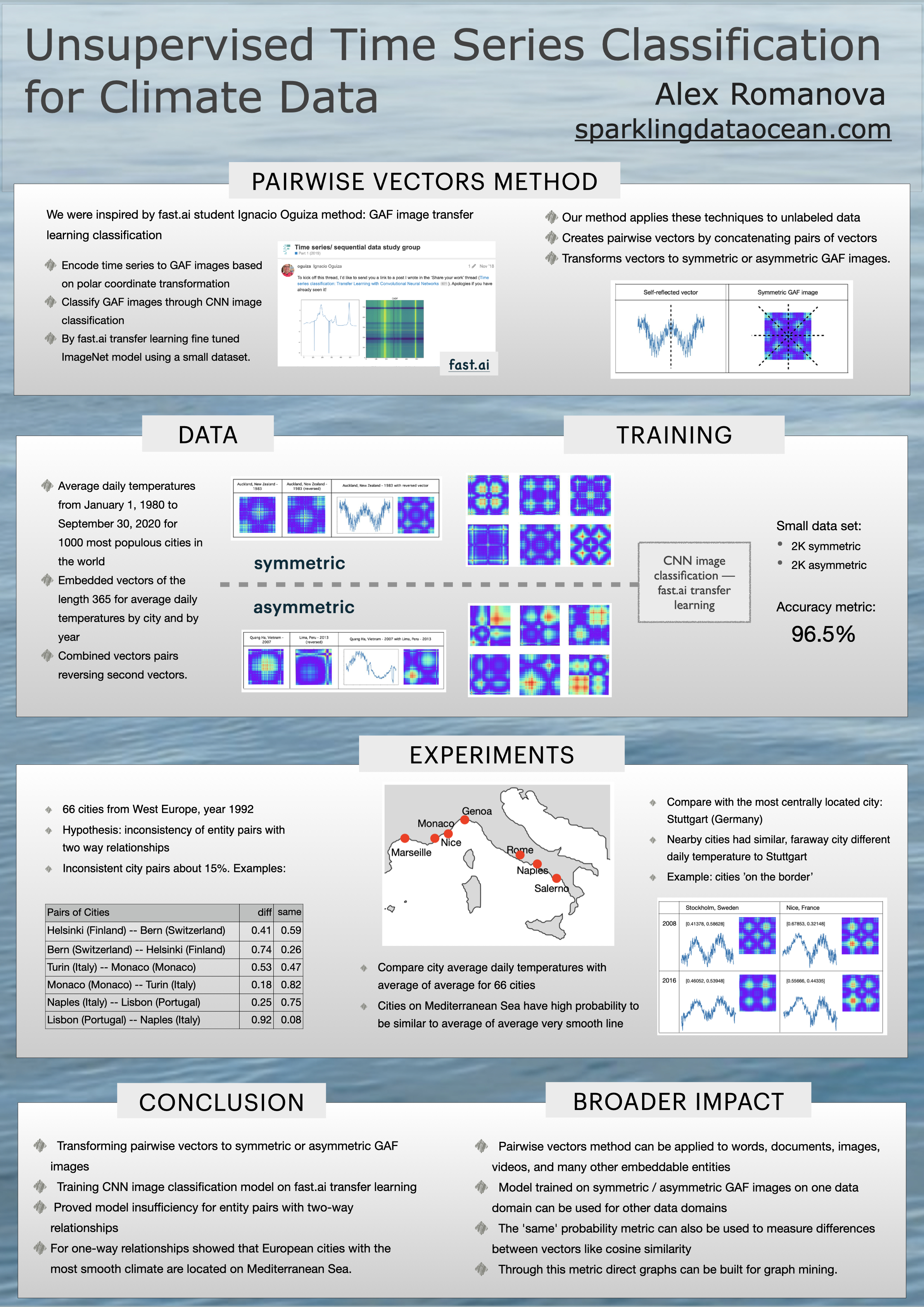
In this post we apply unsupervised machine learning model that categorizes entity pairs to similar pairs and different pairs classes. This is done by transforming pairs of entities to vectors, then vectors to images and classifying images using CNN transfer learning classification.

Previously we used this technique for Natural Language Processing in our post - "Free Associations - Find Unexpected Word Pairs via Convolutional Neural Network" to classify word pairs by word similarities. Based on this model we identified word pairs that are unexpected to be next to each other in documents or data streams. Applying this model to NLP we demonstrated that it works well for classification of entity pairs with one-way relationships. In this post we will show that this model in not reliable to entity pairs with two-way relationships. To demonstrate this we will use city temperature history and will compare temperatures between city pairs.

Methods

Steps that we used for data processing, model training and interpreting the results:

Transformed raw data to embedding vectors
Created pairs of mirror vectors
Transformed mirror vectors to images for CNN image classification
Trained CNN image classification model
Ran mirror vector images through the CNN classification model and analyzed the results

Transform Time Series Data to Mirror Vectors

As the first step of time series data processing we transformed data to embedded vectors that was used as basis for image classification.

Then we generated training data on vector pairs. Second vector in each pair was reversed and vecors were concatenated. We called these concatenated vectors 'mirror vecors'. For ‘Different’ class training data we combined pairs of vectors of different entities and for the 'Same' class training data we combined pairs of vectors of the same entity.

Transform Vectors to Images

As a method of vector to image translation we used Gramian Angular Field (GAF) - a polar coordinate transformation based techniques. We learned this technique in fast.ai 'Practical Deep Learning for Coders' class and fast.ai forum 'Time series/ sequential data' study group. This method is well described by Ignacio Oguiza in Fast.ai forum 'Time series classification: General Transfer Learning with Convolutional Neural Networks'.

To describe vector to GAF image translation Ignacio Oguiza referenced to paper Encoding Time Series as Images for Visual Inspection and Classification Using Tiled Convolutional Neural Networks.

We employed this technique for Natural Language Processing in our two previous posts - "Free Associations - Find Unexpected Word Pairs via Convolutional Neural Network" and "Word2Vec2Graph to Images to Deep Learning."

Training of Unsupervised Vector Classification Model

For this study we used fast.ai CNN transfer learning image classification. To deal with comparatively small set of training data, instead of training the model from scratch, we followed ResNet-50 transfer learning: loaded the results of model trained on images from the ImageNet database and fine tuned it with data of interest. Python code for transforming vectors to GAF images and fine tuning ResNet-50 is described in fast.ai forum.

Python code for transforming vectors to GAF images and fine tuning ResNet-50 is described in Ignacio Oguiza code in his GitHub notebook Time series - Olive oil country.

Data Preparation for Classification

Raw Data

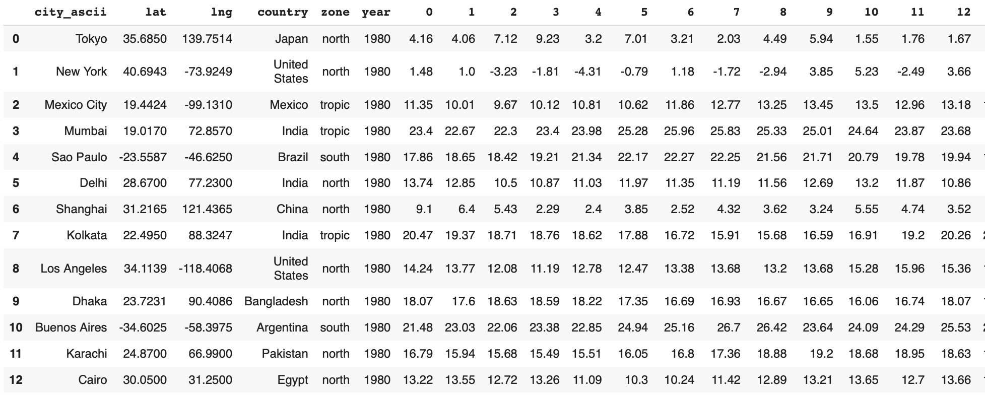
As data Source we will use climate data from Kaggle data sets: "Temperature History of 1000 cities 1980 to 2020" - daily temperature for 1980 to 2020 years from 1000 most populous cities in the world. In our previous post "CNN Image Classification for Climate Data" we described the process of raw data transformation to {city, year} time series:

Metadata columns: city, latitude, longitude, country, zone, year
365 columns with average daily temperatures

Distances Between City Pairs

To analyze results of vector classification we will look for different pairs of vectors from geographically nearby cities and similar pairs for geographically far away cities. First, we will get metadata into cityMetadata table: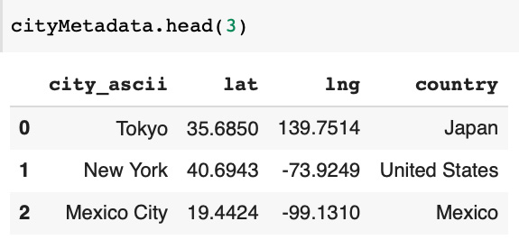

Function to calculate the distance in kilometers by geographic coordinates:

from math import sin, cos, sqrt, atan2, radians
def dist(lat1,lon1,lat2,lon2):
  rlat1 = radians(float(lat1))
  rlon1 = radians(float(lon1))
  rlat2 = radians(float(lat2))
  rlon2 = radians(float(lon2))
  dlon = rlon2 - rlon1
  dlat = rlat2 - rlat1
  a = sin(dlat / 2)**2 + cos(rlat1) * cos(rlat2) * sin(dlon / 2)**2
  c = 2 * atan2(sqrt(a), sqrt(1 - a))
  R=6371.0
  return R * c

Distance between two cities by city metadata and distance fuction:

def cityDist(city1,country1,city2,country2):
  lat1=cityMetadata[(cityMetadata['city_ascii']==city1)
    & (cityMetadata['country']==country1)]['lat']
  lat2=cityMetadata[(cityMetadata['city_ascii']==city2)
    & (cityMetadata['country']==country2)]['lat']
  lon1=cityMetadata[(cityMetadata['city_ascii']==city1)
    & (cityMetadata['country']==country1)]['lng']
  lon2=cityMetadata[(cityMetadata['city_ascii']==city2)
    & (cityMetadata['country']==country2)]['lng']
  return dist(lat1,lon1,lat2,lon2)

Examples of city distances in km:

cityDist('Tokyo','Japan','Mexico City','Mexico')
11301.1797

cityDist('Paris','France','London','United Kingdom')
340.7889

Prepare Vector Pairs

For training data we will create a set 'same' class mirror vecors and 'different' class mirror vectors:

For the 'same' class we will combine vectors with their mirrors
For the 'different' class we will combine random pairs of vectors with temperatures of different years and different cities.
In each pair the second vector will be reversed.

'Same' Class: Coalesce Vectors with their Mirrors

To generate training data images for the 'same' class we will combine vecors with reversed themselves. For each vector we will create a label 'city~year'. For vector pairs we will combine these labels to 'city~year~city~year' labels and will use these labels as file names.

dataSet1 = dataSet.reset_index(drop=True)
dataSet2= dataSet1[dataSet1.columns[::-1]].reset_index(drop=True)
dataSet1['fileName1'] = dataSet1['city_ascii'] + '~' + dataSet1['year'].astype(str)
dataSet1.drop(['city_ascii', 'lat', 'lng','country','zone','year'],
  axis=1, inplace=True)
dataSet2['fileName2'] = dataSet2['city_ascii'] + '~' + dataSet2['year'].astype(str)
dataSet2.drop(['city_ascii', 'lat', 'lng','country','zone','year'],
  axis=1, inplace=True)

Concatenate vectors with reversed themselves
Concatenate 'city~year' labels to 'city~year~city~year' labels
Mark image class type as 'same'.

dataSetSameValues=pd.concat([dataSet1, dataSet2], axis=1)
dataSetSameValues['fileName'] =
  dataSetSameValues['fileName1'] + '~' + dataSetSameValues['fileName2'].astype(str)
dataSetSameValues['type'] ='same'
dataSetSameValues.drop(['fileName1','fileName2'], axis=1, inplace=True)

'Different' Class: Coalesce Vectors with Reversed Other Vectors

To generate training data images for the 'different' class we will do the following steps:

To randomly select different pairs of vectors (dataSet1) we will shuffle vectors and reversed vectors (dataSet2)
For first vectors we will create a label 'city1~year1' and for second (reversed) vectors - label 'city2~year2'
Concatenate vector pairs
Concatenate 'city1~year1' and 'city2~year2' labels to 'city1~year1~city2~year2' labels
Mark image class type as 'different'.

from sklearn.utils import shuffle
dataSet11=shuffle(dataSet1).reset_index(drop=True)
dataSet12=shuffle(dataSet2).reset_index(drop=True)
dataSetDiffValues=pd.concat([dataSet11, dataSet12], axis=1).reset_index(drop=True)
dataSetDiffValues['fileName'] = dataSetDiffValues['fileName1'] + '~' +
  dataSetDiffValues['fileName2'].astype(str)
dataSetDiffValues['type'] ='diff'
dataSetDiffValues.drop(['fileName1','fileName2'], axis=1, inplace=True)

Transform Vectors to Images

Then we will transform mirror vectors to pictures - see more code details in our previous post.

from pyts.image import GramianAngularField as GASF
image_size = 200
gasf = GASF(image_size)
fXcity_gasf = gasf.fit_transform(fXcity)
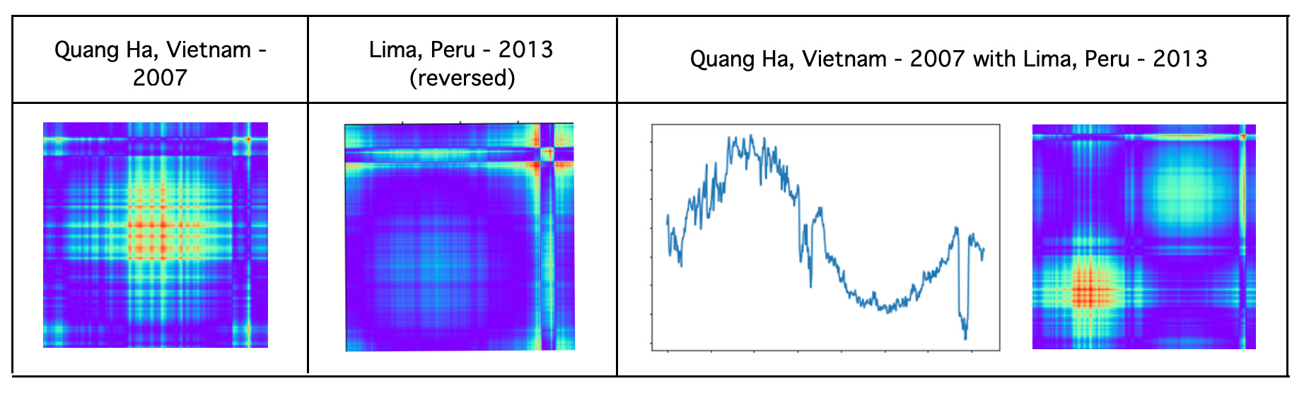
dplt.figure(figsize=(12, 7))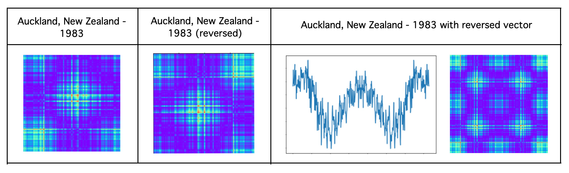

'Same' class example: daily weather in Auckland, New Zealand in 1983.

'Different' class example: daily weather in Quang Ha, Vietnam in 2007 and Lima, Peru in 2013.

For CNN training we will store GAF pictures to 'same' and 'different' subdirectories. Image file names will be defined as labels 'city1~year1~city2~year2'. These file names we will use later for data analysis based on the model results.

imgPath='/content/drive/My Drive/city2'
import os
import warnings
warnings.filterwarnings("ignore")
IMG_PATH = imgPath +'/'+ "img4"
if not os.path.exists(IMG_PATH):
    os.makedirs(IMG_PATH)
numRows=metadataSet.shape[0]
for i in range(numRows):
    if not os.path.exists(IMG_PATH):
        os.makedirs(IMG_PATH)  
    idxPath = IMG_PATH +'/' + str(f['type'][i])
    if not os.path.exists(idxPath):
        os.makedirs(idxPath)
    imgId = (IMG_PATH +'/' +  str(f['type'][i])) +'/' + str(f['fileName'][i])
    plt.imshow(fXpair_gasf[i], cmap='rainbow', origin='lower')  
    plt.savefig(imgId, transparent=True)
    plt.close()

Image Classification Model

Training Data

Prepare data for training and show some 'same' and 'different' class examples.

PATH_IMG=IMG_PATH
tfms = get_transforms(do_flip=False,max_rotate=0.0)
np.random.seed(41)
data = ImageDataBunch.from_folder(PATH_IMG,  train=".", valid_pct=0.20,size=200)
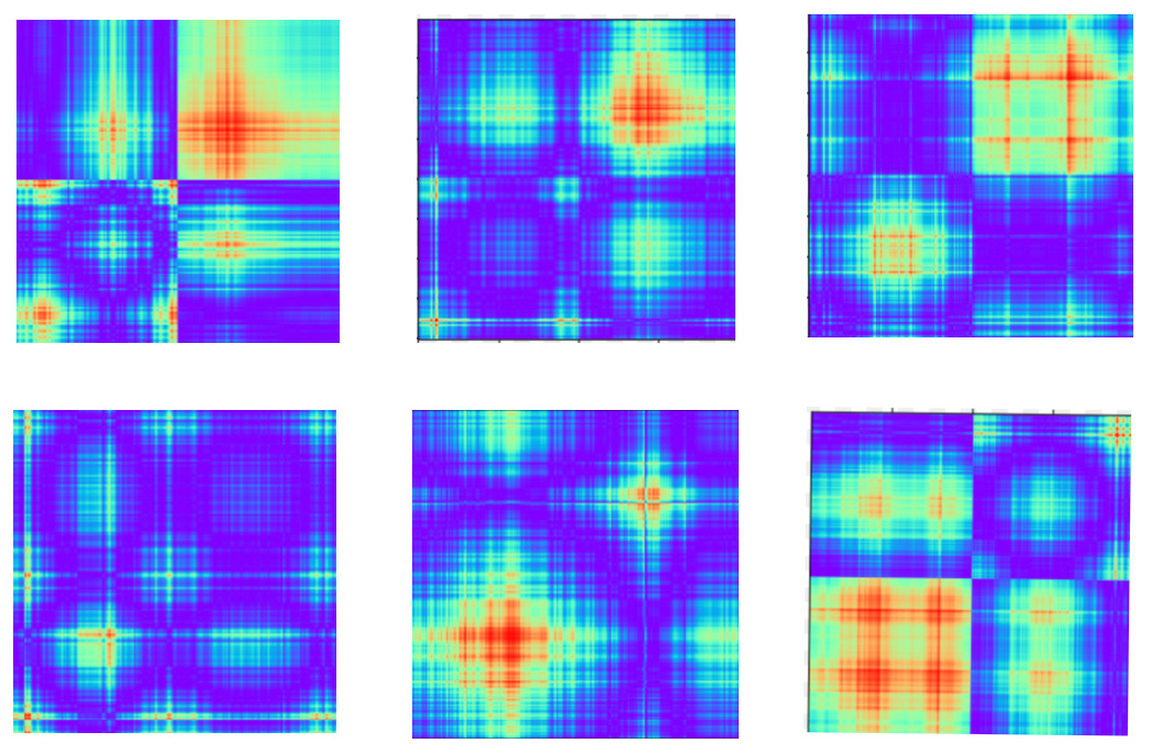
data.show_batch(rows=2, figsize=(9,9))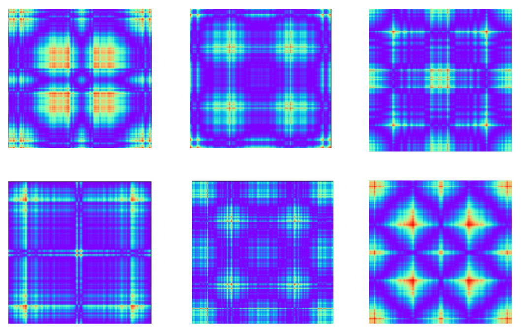

Examples: 'same' class:

Examples: 'different' class:

Train the Model

Time series classification model training was done on fast.ai transfer learning approach:

from fastai.text import *
from fastai.vision import learner
learn = learner.cnn_learner(data, models.resnet34, metrics=error_rate)
learn.fit_one_cycle(2)
learn.save('stage-1a')
interp = ClassificationInterpretation.from_learner(learn)
losses,idxs = interp.top_losses()
len(data.valid_ds)==len(losses)==len(idxs)
interp.plot_top_losses(9, figsize=(10,10))

Accuracy was about 96.5%:

Pairs with Two-way Relationships

Transforming mirror vectors to GAF images technique is based on polar coordinates and therefore it might generate not similar results for turn around pairs. We will test this hypothesis based on the following data:

We will select 66 cities from contitental West Europe and for each city we will take daily temperature data for the year 1992.
For all city pairs we will create mirror vectors in both directions, i.e. Paris - Berlin and Berlin - Paris.
We will transform mirror vectors to GAF images.
Then we will run these images through the model and classify them as 'Similar' or 'Different'.
Finally, we will compare model results for reversed city pairs.

Select Daily Temperature Data for Year 1992 for West European Cities.

Get 1992 year daily temperature data for cities from the following country list:

countryList=['Belgium', 'Germany', 'France','Austria','Netherlands','Switzerland',
              'Spain','Italy','Denmark','Finland','Greece','Italy','Monaco',
              'Netherlands','Norway','Portugal','Sweden','Switzerland']

dataSetEurope = dataSet[(dataSet['country'].isin(countryList))]
dataSet1992 = dataSetEurope[(dataSetEurope['year'].isin(['1992']))]

Combine Pairs of Vectors

Get set of vectors (dataSet21) and transform to reversed vectors (dataSet22).

dataSet21 = dataSet1992.reset_index(drop=True)
dataSet22 = dataSet11[dataSet21.columns[::-1]].reset_index(drop=True)

Attach metadata labels as 'city'~'country'~'year'. To not use the same column names when merging vectors, change dataSet22 column names by adding 'b' prefix.

dataSet21['fileName1'] = dataSet21['city_ascii'] + '~' + dataSet21['country']
  + '~' + dataSet21['year'].astype(str)
dataSet21.drop(['city_ascii', 'lat', 'lng','country','datetime' ,'capital','zone','year'],
  axis=1, inplace=True)
dataSet22['fileName2'] = dataSet22['city_ascii'] + '~' + dataSet22['country']
  + '~' + dataSet22['year'].astype(str)
dataSet22.drop(['city_ascii', 'lat', 'lng','country','datetime', 'capital','zone','year'],
  axis=1, inplace=True)
dataSet23=dataSet22.add_prefix('b')

Merge data frames by keys, exclude self-joined vectors and merge label columns to 'city1'~'country1'~'year1'~'city2'~'country2'~'year2':

dataSet21['key']=0
dataSet23['key']=0
pairDataSet = dataSet21.merge(dataSet23,on='key', how='outer')
pairDataSet2 = pairDataSet[pairDataSet['fileName1']!=pairDataSet['bfileName2']]
pairDataSet2['fileName'] = pairDataSet2['fileName1'].astype(str)
  + '~' + pairDataSet2['bfileName2'].astype(str)
pairDataSet2.drop(['fileName1','bfileName2','key'], axis=1, inplace=True)

Transform Vectors to GAF Images

Split data set to vectors and labels:

mirrorDiffColumns = pairDataSet2[['fileName']]
dataSetPairValues = pairDataSet2.drop(pairDataSet3.columns[[730]],axis=1)

Transform vectors to images and save images using label (fileName) as image name:

fXpair=dataSetPairValues.fillna(0).values.astype(float)
image_size = 200
gasf = GASF(image_size)
fXpair_gasf = gasf.fit_transform(fXpair)
IMG_PATH = '/content/drive/My Drive/city2/img9'
numRows = mirrorDiffColumns.shape[0]
for i in range(numRows):
   imgId = (IMG_PATH +'/' +  str(f['fileName'][i]))
   plt.imshow(fXpair_gasf[i], cmap='rainbow', origin='lower')  
   plt.savefig(imgId, transparent=True)
   plt.close()

Vector Classification Based on the Model

To predict vector similarities based on the trained model, we will use fast.ai function 'learn.predict':

PATH_IMG='/content/drive/My Drive/city2/img4'
data = ImageDataBunch.from_folder(PATH_IMG,  train=".", valid_pct=0.23,size=200)
learn = learner.cnn_learner(data2, models.resnet34, metrics=error_rate)
learn.load('stage-1a')

Here are two examples of city pairs. The first number shows 'different' probability and second number - 'same' probability:

pred_class,pred_idx,out=learn.predict(open_image(str(
  '/content/drive/MyDrive/city2/img9/Marseille~France~1992~Paris~France~1992.png')))
pred_class,pred_idx,out
(Category tensor(0), tensor(0), tensor([0.8589, 0.1411]))

pred_class,pred_idx,out=learn.predict(open_image(str(
  '/content/drive/MyDrive/city2/img9/Turin~Italy~1992~Monaco~Monaco~1992.png')))
pred_class,pred_idx,out
(Category tensor(0), tensor(0), tensor([0.5276, 0.4724]))

The following example shows that temperature similarities depend on city order. In the first result vectors in Naples and Porto are 'same' but vectors between Porto and Naples are 'different':

pred_class,pred_idx,out=learn.predict(open_image(str(
  '/content/drive/MyDrive/city2/img9/Naples~Italy~1992~Porto~Portugal~1992.png')))
pred_class,pred_idx,out
(Category tensor(1), tensor(1), tensor([0.3950, 0.6050]))

pred_class,pred_idx,out=learn.predict(open_image(str(
  '/content/drive/MyDrive/city2/img9/Porto~Portugal~1992~Naples~Italy~1992.png')))
pred_class,pred_idx,out
(Category tensor(0), tensor(0), tensor([0.6303, 0.3697]))

To calculate how many inconsistent pairs we have, first, we will run all images through the model:

pathPair='/content/drive/MyDrive/city2/img9/'
files = os.listdir(pathPair)
resEI1992=[]
for file in files:
  pred_class,pred_idx,out=learn.predict(open_image(pathPair +  '/' +file))
  resEI1992.append((file,out[0].tolist(),out[1].tolist()))
dfRes1992EIdata = DataFrame (resEI1992,columns=['cityPair','probDiff','probSame'])

dfRes1992EIdata.shape
(4290, 4)

Next, we will split 'cityPair' column to {city, country, year} pairs:

dfRes1992EIdata[['city1','country1','year','city2','country2','xx']] =
  dfRes1992EIdata.cityPair.apply(lambda x: pd.Series(str(x).split("~")))

Calculate distances (in kilometers) between cities:

cityMetadataPath='/content/drive/MyDrive/city1/img6/cityMetadata.csv'
cityMetadata=pd.read_csv(cityMetadataPath,sep=',',header=0).
  drop(['Unnamed: 0','datetime','zone'],axis=1)
dfRes1992EIdata['dist'] = dfRes1992EIdata.
  apply(lambda x: cityDist(x.city1,x.country1,x.city2,x.country2), axis=1)
dfRes1992EIdata=dfRes1992EIdata.drop(['Unnamed: 0','cityPair','xx'],axis=1)

Finally, the total number of city pairs we have is 4290 and there are 630 inconsisted city pairs, therefore about 14.7% of city pairs get inconsisted model results.

dfRes1992EIdata['same']=(0.5-dfRes1992EIdata.probSame)*(0.5-dfRes1992EIdata.probSame2)

len(dfRes1992EIdata.loc[dfRes1992EIdata['same'] < 0])
630

Inconsistency of city pairs similarity predictions are not dependent of distances between the cities: this problem occurs for city pairs that are located nearby and faraway. For example, here are city pairs with inconsisted similarity predictions and longest distances:

dfRes1992EIdata.loc[dfRes1992EIdata['same'] < 0].sort_values('dist').tail(18)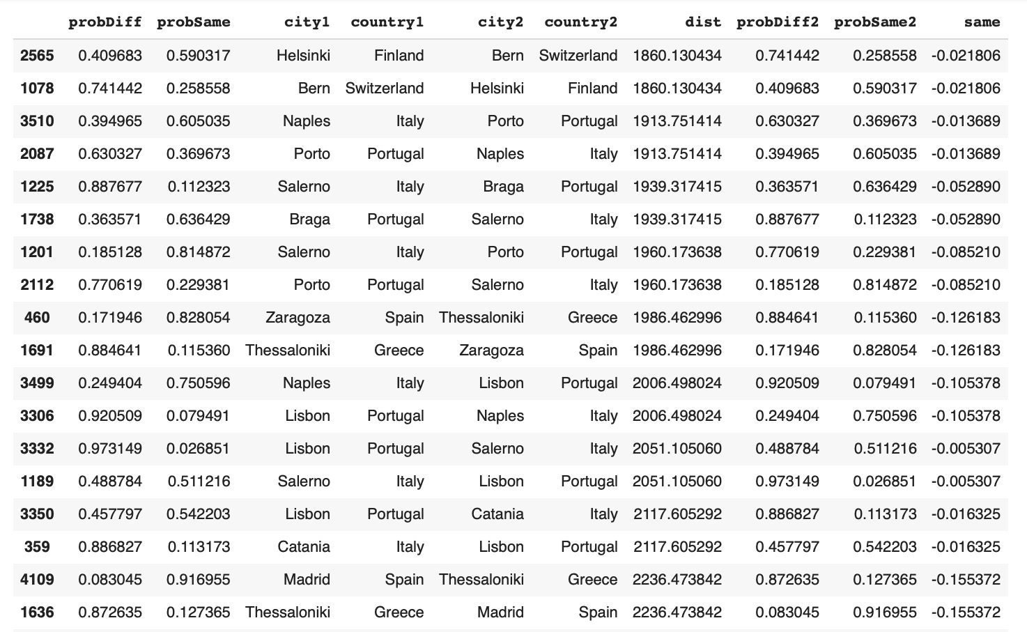

Examples of city pairs with inconsisted similarity predictions and shortest distances:

dfRes1992EIdata.loc[dfRes1992EIdata['same'] < 0].sort_values('dist').head(18)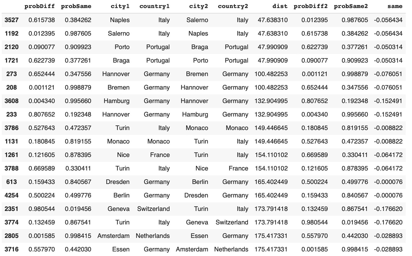

Find Outliers

We proved the hypothesis that mirror vectors classification model is not reliable for similarity prediction of pairs with two-way relationships and therefore this model should be used only for classifcation of entity pairs with one-way relationships.

Here we will show scenarios of using this model to compare daily temperatures of pairs with one-way relationships. First, we will calculate average vector of all yearly temperatures vectors for cities in Western Europe and compare it with yearly temperature vectors for all cities. Second, we will find a city located in the center of Western Europe and compare this city temperatures for years 2008 and 2016 with other cities.

Compare {City, Year} Temperature Vectors with Average of All Yearly Temperatures

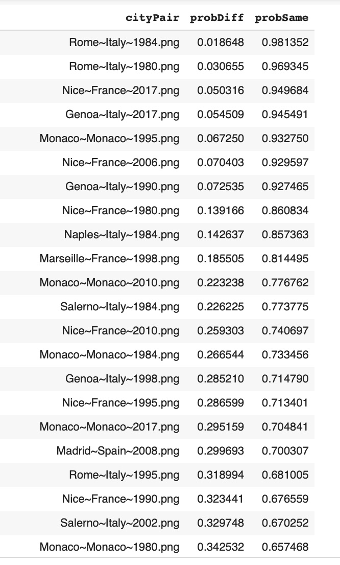
To find cities with yearly temperatures similar to average temperatures for years from 1980 to 2019 in Western Europe we calculated average time series for 2640 daily temperature time series (40 years and 66 cities).

As average of average temperature vectors provides a very smooth line, we don't expect that many city-year temperature vectors will be similar to it. In fact only 33 of city-year temperature time series (1.25%) had higher than 0.5 'same' probability. Here are top 22 pairs with 'same' probability higher than 0.65:

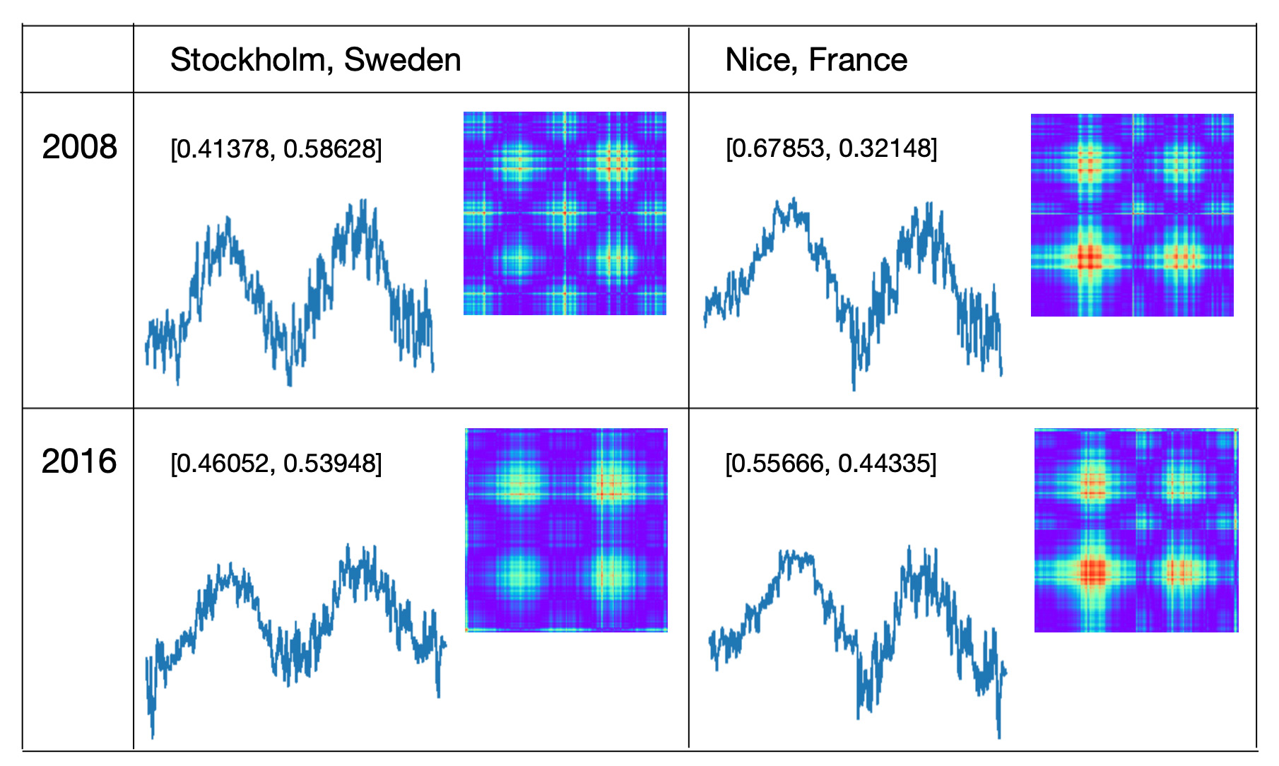
It's interesting that most of cities with high probabilities to be similar to average temperature are located on Mediterranean Sea not far from each other. Here is a clockwise city list: Marseille (France), Nice (France), Monako (Monako), Genoa (Italy), Rome (Italy), Naples (Italy), and Salerno (Italy).

Compare {City, Year} Temperature Vectors with Central City

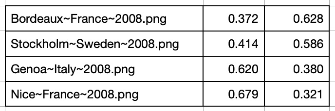
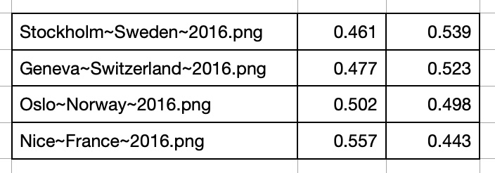
Here is another scenario of using mirror vector model to compare daily temperatures of pairs with one-way relationships. From Western Europe city list the most cetrally located city is Stuttgart, Germany.

Concatenated temperature vector pairs {city, Stuttgart} for years 2008 and 2016
Transformed mirror vectors to GAF images
Analyzed 'same' or 'different' probabilities by running images through trained model.

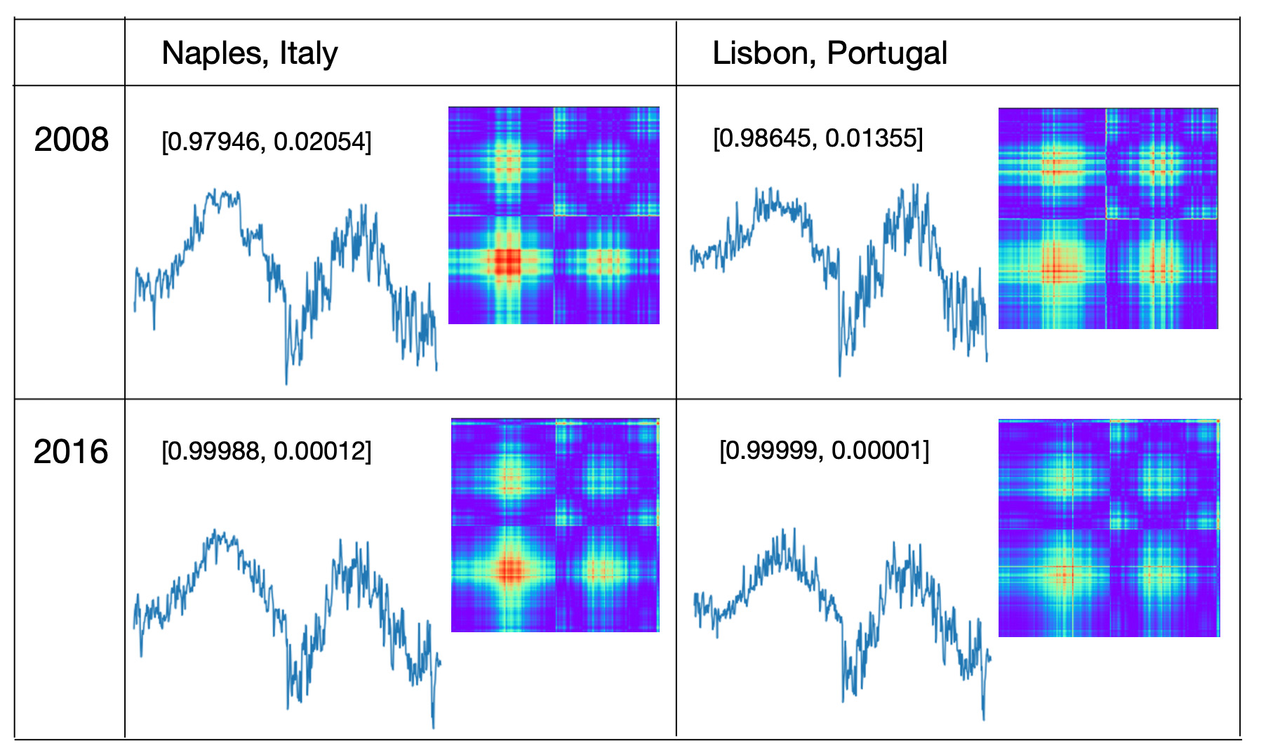
Based on the model, for both years, cities located close to Stuttgart had high probability of similar temperature vectors and cities located far from Stuttgart had high probabilities of different temperature vectors. Here we show two cities that had very different temperatures in both 2008 and 2016 years:

Less easy was to predict which cities had temperature vector similarities on the border between 'different' and 'same'. Here are cities for the year 2008:

And here are cities for the year 2016:

Here are two cities that were 'on the border' in years 2008 and 2016. In both years Stockholm, Sweden was on the 'same' side and Nice, France was on 'different' side.

Presentation on NLDL2022 Conference

This study was presented on "Northern Lights Deep Learning Conference (NLDL2022)" conference.