CNN Image Classification for Climate Data

Convolutional Neural Network Classification Methods

Outstanding success of Convolutional Neural Network image classification in the last few years influenced application of this technique to extensive variety of objects. In particular, deep learning techniques became very powerful after evolutionary model AlexNet was created in 2012 to improve the results of ImageNet challenge. Since the introduction of large-scale visual datasets like ImageNet, most success in computer vision has been primarily driven by supervised learning.

CNN image classification methods are getting high accuracies but being based on supervised machine learning, they require labeling of huge volumes of data. One of the solution of this challenge is transfer learning. Fine-tuning a network with transfer learning usually works much faster and has higher accuracy than training CNN image classification models from scratch.

In this post we examine how to apply CNN image classification transfer learning methods to climate data analysis.

CNN Classification of Embedded Vectors

In this post we will use a deep learning technique that we learned in fast.ai 'Practical Deep Learning for Coders, v3' class and fast.ai forum 'Time series/ sequential data' study group.

In our previous posts we employed this technique to Natural Language Processing - "Free Associations - Find Unexpected Word Pairs via Convolutional Neural Network" and "Word2Vec2Graph to Images to Deep Learning." and to electroencephalography data analysis: "EEG Patterns by Deep Learning and Graph Mining."

CNN Classification Method

For classification method we will convert yearly daily temperature datas to images using Gramian Angular Field (GASF) - a polar coordinate transformation. This method is well described by Ignacio Oguiza in Fast.ai forum 'Time series classification: General Transfer Learning with Convolutional Neural Networks'. He referenced to paper Encoding Time Series as Images for Visual Inspection and Classification Using Tiled Convolutional Neural Networks. For data processing we will use ideas and code from Ignacio Oguiza code is in his GitHub notebook Time series - Olive oil country.

Data Preprocessing

Data Source

To demonstrate how this methods work we will use climate data from kaggle.com data sets: "Temperature History of 1000 cities 1980 to 2020".

This data has average daily temperature in Celsius degrees for years from January 1, 1980 to September 30, 2020 for 1000 most populous cities in the world.

Transform Raw Data to Daily Temperature by Year Vectors

The raw data of average daily temperature for 1000 cities is represented in 1001 columns - city metadata and average temperature rows for all dates from 1980, January 1 to September 30, 2020.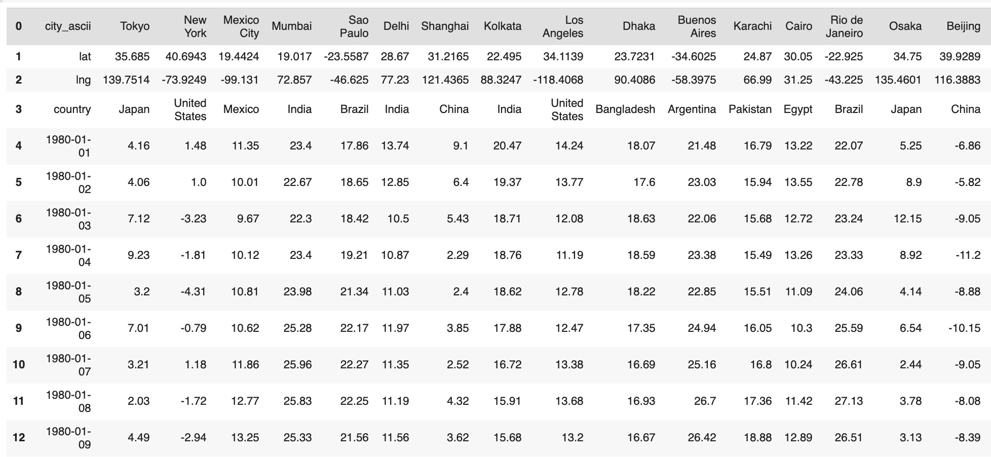

To experiment with classification method we'll calculate 'zone' metadata as Tropical, North and South regions based on latitude:

cityMetadata['lat']=pd.to_numeric(cityMetadata['lat'])
cityMetadata['lng']=pd.to_numeric(cityMetadata['lng'])
cityMetadata['zone'] = 'tropic'
cityMetadata['zone'][cityMetadata['lat'] > 23.5] = 'north'
cityMetadata['zone'][cityMetadata['lat'] < -23.5] = 'south'

As city metadata we will use the following columns:

City
Country
Latitude
Longitude
Zone

We will convert raw data to set of embedded vectors {city, year}:

To get the same data format for each time series from raw data we excluded February 29 rows
As we had data only until September 30, 2020, we excluded data for year 2020
From dates formated as 'mm/dd/yyyy' strings we extracted year as 'yyyy' strings

tempCity3=tempCity2[~(tempCity2['metadata'].str.contains("2020-"))]
tempCity4=tempCity3[~(tempCity3['metadata'].str.contains("-02-29"))]
tempCity4['metadata']=tempCity4['metadata'].str.split(r"-",n=0,expand=True)
tempCity4=tempCity4.reset_index(drop=True)

Next, we transformed data to the following structure:

Metadata columns: city, latitude, longitude, country, zone, year
365 columns with average daily temperatures

tempCityGroups=tempCity5.groupby(['metadata'])
dataSet=pd.DataFrame()
for x in range(1980, 2020):
  tmpX=tempCityGroups.get_group(str(x)).reset_index(drop=True)
  tmpX=tmpX.drop(tmpX.columns[[0]],axis=1).T
  cityMetadata['year']=x  
  cityMetadata.reset_index(drop=True, inplace=True)
  tmpX.reset_index(drop=True, inplace=True)
  df = pd.concat( [cityMetadata, tmpX], axis=1)
  dataSet=dataSet.append(df)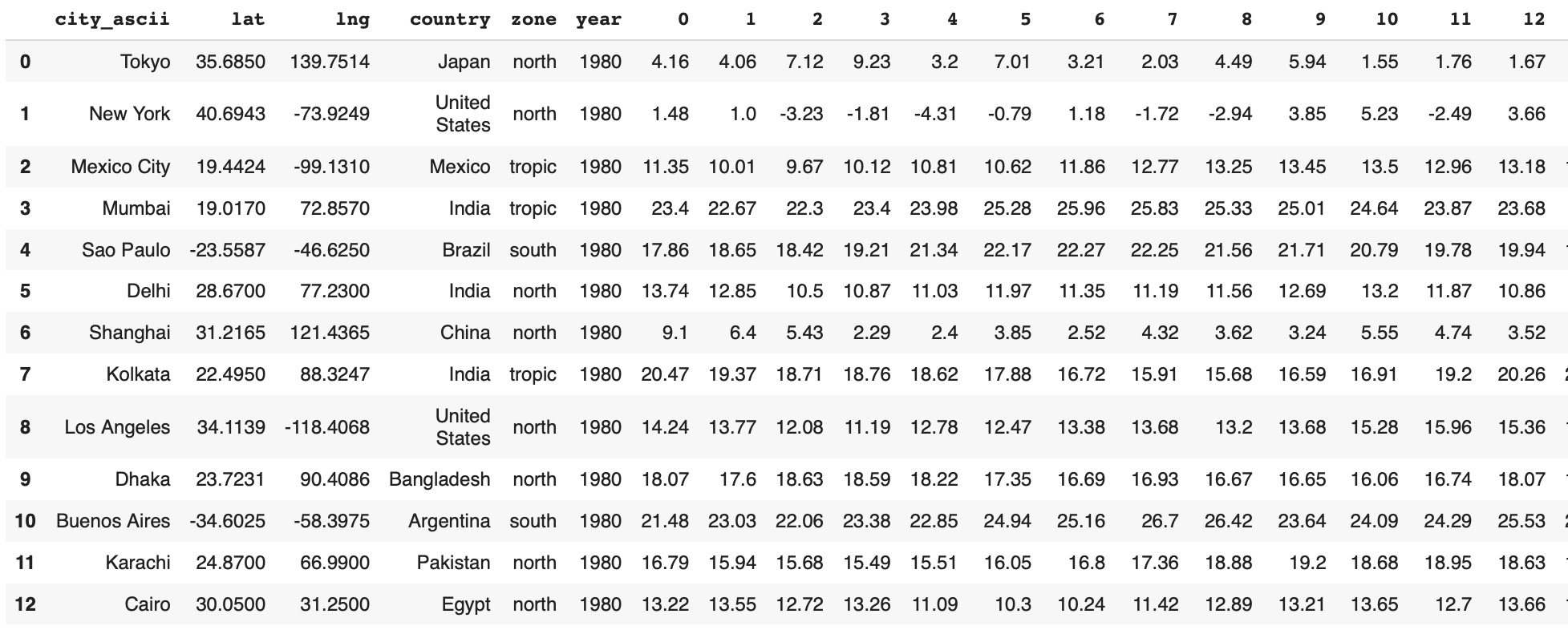

Prepare Training Data by Zone

We will classify daily temperature time series by North, South and Tropical zones. The distribution of populated cities is not proportional by zones: about one third of cities are located in Tropical region, much more on Northern region and much less on Southern region:

Northern region: 614 cities
Tropical region: 340 cities
Sourthern region: 46 cities

To get similar sizes of training data by regions we will take all information for South region (1840 records) and randomly select about 2000 records for North and Tropical regions.

Data Prearation for Southern Region

We will describe in detail data preparation process for Southern region. For the other two regegions data preparation processes are very similar. As in raw data we have only 46 cities in Southern region, we will use all this data for training. Here are the following steps:

Transforn temperature values from string format to float format
Get a subset of data for Southern region
Split data to metadata and data values
Transform data values to numpy format
Transform daily temperature float arrays to pictures

dataSet = dataSet.reset_index(drop=True)
dataSet.iloc[:,6:] = dataSet.iloc[:,6:].astype(float)
dataSetSouth=dataSet[dataSet['zone']=="south"]
dataSetSouth = dataSetSouth.reset_index(drop=True)
metadataSet=dataSetSouth.iloc[:,:7]
dataValues=dataSetSouth.drop(dataSetSouth.columns[[0,1,2,3,4,5,6]],axis=1)
fXcity=dataValues.fillna(0).values.astype(float)
from pyts.image import GramianAngularField as GASF
image_size = 200
gasf = GASF(image_size)
fXcity_gasf = gasf.fit_transform(fXcity)
dplt.figure(figsize=(12, 7))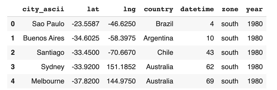

To illustrate examples of images that will be used as training data, we will look at Southern region metadata, select city and year and draw pictures. Here we picked up a row with index=1 from Southern region metadata and draw plot and GASF images for daily weather data in Buenos Aires in 1980:

plt.plot(fXcity[1])
plt.imshow(fXcity_gasf[1], cmap='rainbow', origin='lower')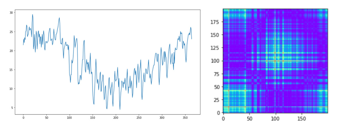

Next, we will transform all {city, year} time series to GASF pictures and store them in 'south' subdirectory. As the name of images we will use combinations of city names and years:

imgPath='/content/drive/My Drive/city1'
import os
import warnings
warnings.filterwarnings("ignore")
IMG_PATH = imgPath +'/'+ "img10"
if not os.path.exists(IMG_PATH):
    os.makedirs(IMG_PATH)
numRows=metadataSet.shape[0]
for i in range(numRows):
    if not os.path.exists(IMG_PATH):
        os.makedirs(IMG_PATH)  
    idxPath = IMG_PATH +'/' + str(metadataSet['zone'][i])
    if not os.path.exists(idxPath):
        os.makedirs(idxPath)
    imgId = (IMG_PATH +'/' +  
      str(metadataSet['zone'][i])) +'/' +
      str(metadataSet['city_ascii'][i]+'~'+
      str(metadataSet['year'][i]))
    plt.imshow(fXcity_gasf[i], cmap='rainbow', origin='lower')   
    plt.savefig(imgId, transparent=True)
    plt.close()

Tropical and North Regions

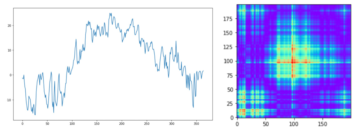
For Tropical and Northern regions we will shuffle data and select about 2000 rows. Southern region example: plot and GASF images for daily weather data in Singapore in 1999.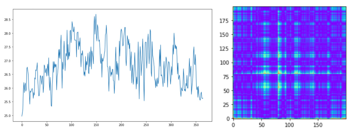

Northern region example: plot and GASF images for daily weather in Moscow in 2013.

Immage Classification

Training Data Preparation

For time series classification model we used transfer learning approach from fast.ai library. Here is code to prepare data for model training and and show some Southern region data examples:

PATH_IMG=IMG_PATH
tfms = get_transforms(do_flip=False,max_rotate=0.0)
np.random.seed(41)
data = ImageDataBunch.from_folder(PATH_IMG,  train=".", valid_pct=0.20,size=200)
data.show_batch(rows=3, figsize=(9,9))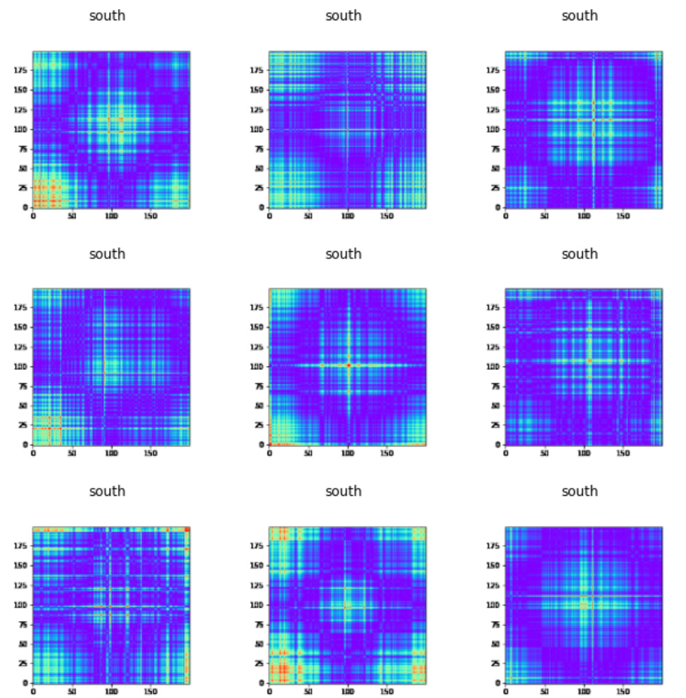

Model Training

Code based on fast.ai library to train the time series classification model and save the results:

from fastai.text import *
from fastai.vision import learner
learn = learner.cnn_learner(data, models.resnet34, metrics=error_rate)
learn.fit_one_cycle(2)
learn.save('stage-1a')

Interpretation of CNN Classification Model

interp = ClassificationInterpretation.from_learner(learn)
losses,idxs = interp.top_losses()
len(data.valid_ds)==len(losses)==len(idxs)
interp.plot_top_losses(9, figsize=(10,10))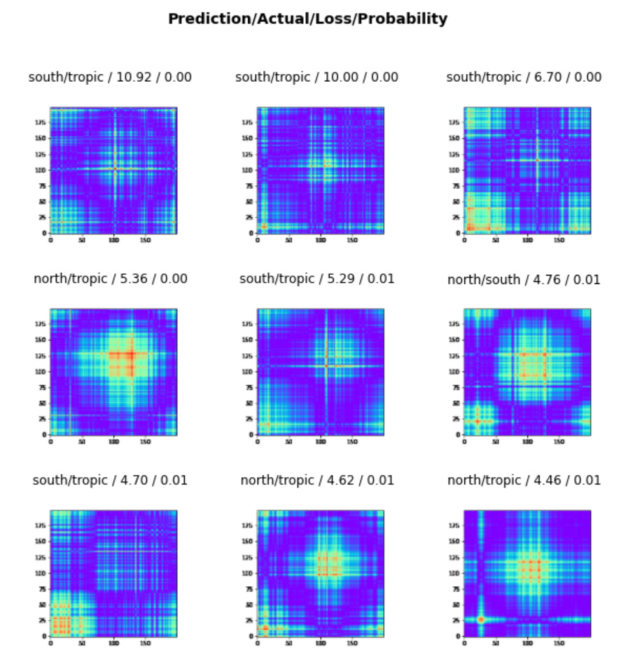

interp.most_confused(min_val=2)
[('tropic', 'north', 32),
 ('tropic', 'south', 16),
 ('south', 'north', 14),
 ('north', 'tropic', 12),
 ('south', 'tropic', 9),
 ('north', 'south', 6)]  

interp.plot_confusion_matrix(figsize=(6,6), dpi=60)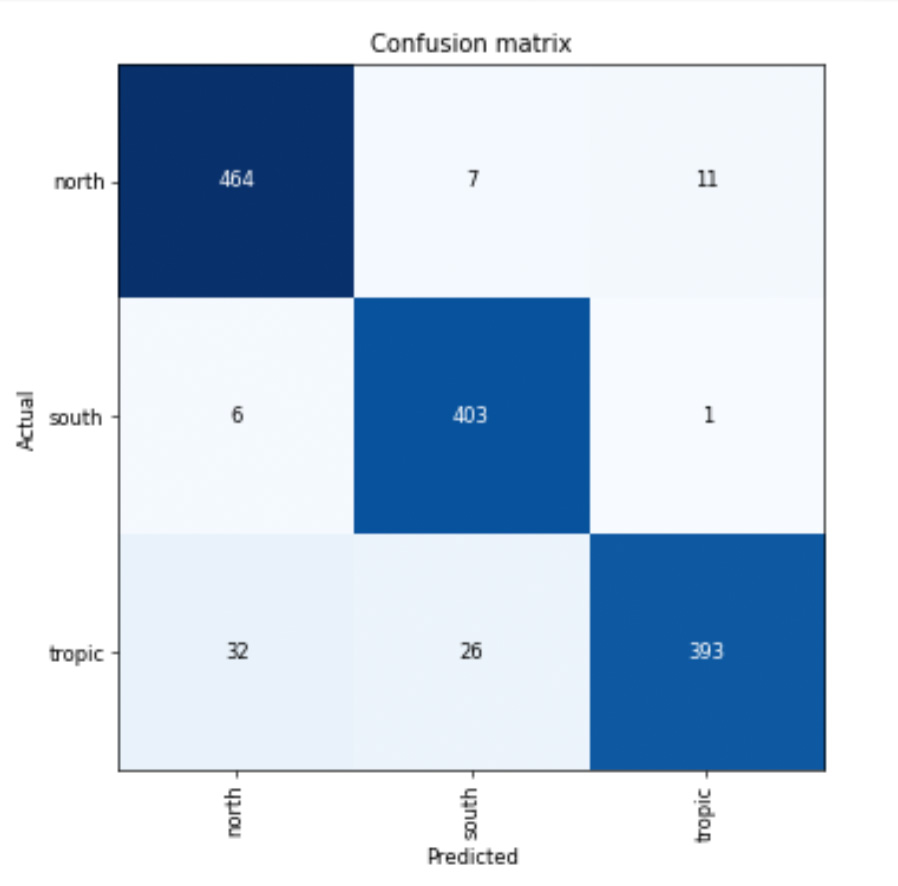

CNN Model Accuracy Statistics

The error rate of the model is 6.8% and the arccuracy about 93.8%.

To calculate accuracy statistics we'll read the data and run it through the model and split the results by zone:

path7='/content/drive/MyDrive/city1/img10/'
dirs7 = os.listdir( path7 )
cityList=[]
res7=[]
for zone in ['north','south','tropic']:
  dirZone= os.listdir( path7 + zone)
  for file in dirZone:
    cityList.append(path7 + zone + '/' +file)
    pred_class,pred_idx,out=learn.predict(open_image(path7 + zone + '/' +file))
    res7.append((zone,file,out[0].tolist(),out[1].tolist(),out[2].tolist()))
dfResZone = DataFrame (res7,columns=['zone','file','predNorth','predSouth','predTropic'])
cityYearProbTropic=cityYearProb[cityYearProb['zone']=='tropic']
cityYearProbSouth=cityYearProb[cityYearProb['zone']=='south']
cityYearProbNorth=cityYearProb[cityYearProb['zone']=='north']

For each table we calculated statistics:

cityYearProbTropic.describe()
        predNorth	predSouth	predTropic	lat	        lng
count	2017.000000	2017.000000	2017.000000	2017.000000	2017.000000
mean	0.069153	0.024727	0.906120	6.760149	28.098896
std	0.168732	0.116081	0.203176	12.707139	77.334275
min	0.000014	0.000008	0.000018	-23.490000	-175.220600
25%	0.000592	0.000175	0.941811	-2.980000	-45.879900
50%	0.003178	0.000662	0.993542	9.935000	37.340000
75%	0.029660	0.003441	0.998776	17.400000	100.329400
max	0.993994	0.999964	0.999953	23.489500	179.216600

Then we combined resuls by taking north region probability ('predNorth' column) for Northern region statistics, tropic region probability for Tropical region statistics and south region probability for Southern region.

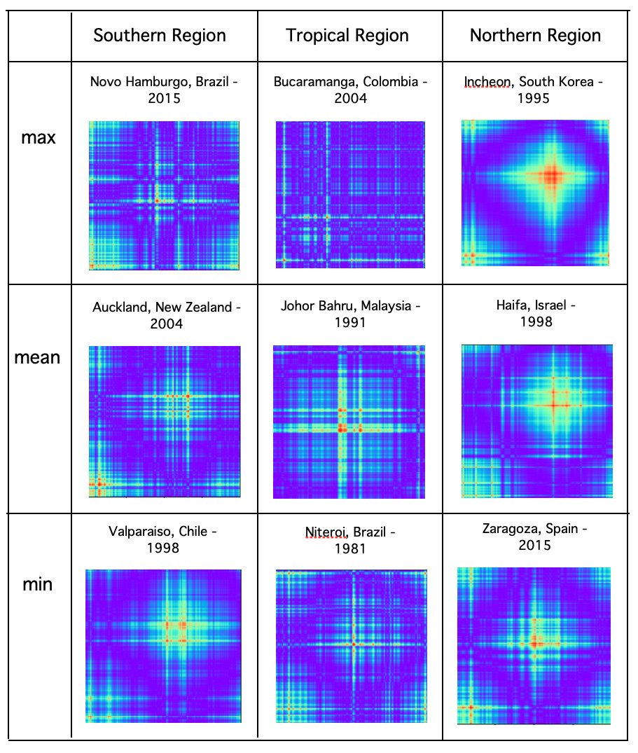
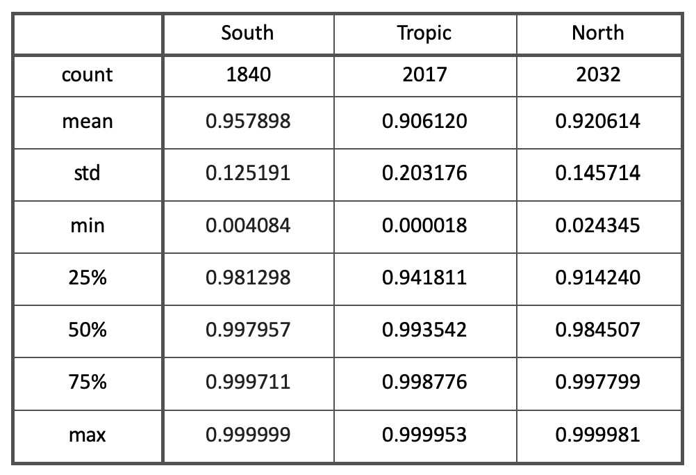Here are max, min and mean image examples for Northern, Southern and Tropical regions:

Next Post - Unsupervised Learning

In the next post we will show how to build unsupervised learning CNN image classification model.