Word2Vec2Graph to Images to Deep Learning

Vector Classification

In this post we will play with another amazing deep learning technique about Time Series classification via CNN Deep Learning. We learned this technique in fast.ai 'Practical Deep Learning for Coders, v3' class and fast.ai forum 'Time series/ sequential data' study group.

We will analyze a long document, uncover new topics (clusters) and use CNN classification as a validation method for graph clustering.

To find topics in long text file we will build Word2Vec2Graph on top of Word2Vec model. Document words will be used as graph nodes and cosine similarities between word vectors as edge weights for this graph. The Word2Vec2Graph model is described in details in previous posts of this blog.

Word vectors will be transformed to images using method described in notebook created by Ignacio Oguiza Time series - Olive oil country. As different clusters we will use topics generated from Word2Vec2Graph graph. Than we will use CNN classification model to validate clustering:

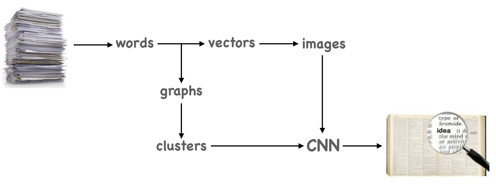
In particular, we will use CNN classification model to prove that topic we discover are different. This validation method will not let us to get rid of noise in our clusters: if two words are in the same cluster it does not mean that they are highly connected. But if two words are in different clusters they obviously do not belong to the same topic.

Data Preparation

Data preparation process for Word2Vec2Graph model in described in previous posts and summarized in the "Word2Vec2Graph - Insights" post. Here we used the same data preparation process of text data about Creativity and Aha Moments:Word2Vec2Graph - Insights

Read text file
Tokenize
Remove stop words
Read trained Word2Vec model
Build a graph with words as nodes and cosine similarities as edge weights.
Save graph vertices and edges

Read and Clean File about Creativity and Aha Moments

Read text file, tokenize it and remove stop words:

import org.apache.spark.ml._
import org.apache.spark.ml.feature._
import org.apache.spark.sql.functions.explode
import org.apache.spark.ml.feature.Word2Vec
import org.apache.spark.ml.feature.Word2VecModel
import org.apache.spark.sql.Row
import org.apache.spark.ml.linalg.Vector
import org.graphframes.GraphFrame
import org.apache.spark.sql.DataFrame
import org.apache.spark.sql.expressions.Window
import org.apache.spark.sql.functions._
import org.apache.spark.sql.functions.explode
val tokenizer = new RegexTokenizer().
   setInputCol("charLine").
   setOutputCol("value").
   setPattern("[^a-z]+").
   setMinTokenLength(5).
   setGaps(true)
val inputInsight=sc.
   textFile("/FileStore/tables/ahaMoments.txt").
   toDF("charLine")
val tokenizedInsight = tokenizer.
   transform(inputInsight)
val remover = new StopWordsRemover().
   setInputCol("value").
   setOutputCol("stopWordFree")
val removedStopWordsInsight = remover.
   setStopWords(Array("none","also","nope","null")++
   remover.getStopWords).
   transform(tokenizedInsight)
val slpitCleanInsight = removedStopWordsInsight.
   withColumn("cleanWord",explode($"stopWordFree")).
   select("cleanWord").
   distinct

Read trained Word2Vec model and from data about Creativity and Aha Moments text exclude words that are not in the model:

val word2vec= new Word2Vec().
   setInputCol("value").
   setOutputCol("result")
val modelNewsBrain=Word2VecModel.
   read.
   load("w2VmodelNewsBrain")
val modelWordsInsight=modelNewsBrain.
   getVectors.
   select("word","vector")
val cleanInsight=slpitCleanInsight.
   join(modelWordsInsight,'cleanWord==='word).
   select("word","vector").
   distinct

Build a Graph and Find Topics

Read nodes and edges that we calculated and saved before, build a graph with words as nodes and cosine similarities as edge weights. How to build the graph was described in details in our post "Introduction to Word2Vec2Graph Model."

val graphInsightVertices = sqlContext.read.parquet("graphVerticesSub")
val graphInsightEdges = sqlContext.read.parquet("graphEdgesSub")
val graphInsight2 = GraphFrame(graphInsightVertices, graphInsightEdges)
graphInsight2.persist

Function to calculate connected components with cosine similarly and component size parameters:

def word2vector2ghraphCCid(graphVertices: DataFrame, graphEdges: DataFrame,
     cosineMin: Double, cosineMax: Double):
  DataFrame = {
  val graphEdgesSub= graphEdges.filter('edgeWeight>cosineMin).filter('edgeWeight<cosineMax)
  val graphSub = GraphFrame(graphVertices, graphEdgesSub)
  sc.setCheckpointDir("/FileStore/")
  val resultCC = graphSub.
     connectedComponents.
     run()
  val resultCCcount=resultCC.
     groupBy("component").
     count.
     toDF("cc","ccCt")
  resultCC.join(resultCCcount,'component==='cc).    
     select("id","component","ccCt").distinct
}

Calculate connected components with high cosine similarly:

val resultsCCid=word2vector2ghraphCCid(graphInsightVertices, graphInsightEdges,0.8, 0.99)

display(resultsCCid.select("component","ccCt").distinct.orderBy('ccCt.desc))
   component	ccCt
  8589934606	 315
          19	  80
           2	  70
 60129542151	  52
 17179869190	  44
 25769803789	  12
 34359738374	   8
180388626448	   7
455266533384	   7

Calculate Top PageRanks for Connected Components

Calculate graph Page Ranks:

val graphSub2PageRank = graphInsight2.
   pageRank.
   resetProbability(0.15).
   maxIter(11).
   run()
display(graphSub2PageRank.vertices.
   distinct.
   sort($"pagerank".desc))

id     pagerank
funny    4.66
costumes    3.92
weird    3.82
brandon     3.60
integrated    3.52
symptoms    3.37
decrease    3.35
craig     3.27
bruce    3.19

Join PageRank data with connected components and find the top Page Rank word for each component:

val graphCCpageRank=graphSub2PageRank.vertices.
   join(resultsCCid.filter("ccCt>12") ,Seq("id"))

val partitionWindow = Window.partitionBy($"component").
   orderBy($"pageRank".desc)
val ccTopPageRank = graphCCpageRank.
   withColumn("ccPageRank", rank().over(partitionWindow)).
   select("id","component").toDF("topCCword","componentId")

display(ccTopPageRank.filter("ccPageRank=1"))
   topCCword	componentId
   decrease	19
   emory	17179869190
   integrated	2
   funny	8589934606
   symptoms	60129542151

Use the top PageRank as a class word for connected components:

val classWords=resultsCCid.filter("ccCt>12").
   join(ccTopPageRank.filter("ccPageRank=1"),'component==='componentId).
   withColumn("classWord",concat($"topCCword",lit("~"),$"ccCt")).
   select("classWord","id")

Define word vectors, convert vectors to strings and save it as csv file:

val cc2vec=classWords.join(modelWordsInsight,'id==='word).drop("word").
   map(s=>(s(0).toString,s(1).toString,s(2).toString)).
   toDF("class","classWord","vec").
   withColumn("vec2",regexp_replace($"vec","\\["," ")).drop("vec").
   withColumn("vecString",regexp_replace($"vec2","\\]"," ")).drop("vec2")

class,classWord,vecString
integrated~70,solutions," -0.14655259251594543,-0.0015149622922763228,-0.21045255661010742,0.02907191775739193,-0.010674788616597652,0.08036941289901733,
   0.010507240891456604,-0.17006824910640717,0.11951962113380432,-0.14497050642967224,-0.0026977339293807745,0.04952468350529671,0.2884736657142639,-0.05758485198020935,-0.1312779188156128,0.024382397532463074,0.008873523212969303,0.1334419697523117,-0.031296879053115845,0.015222832560539246,-0.05807945132255554,0.09823902696371078,-0.15477193892002106,0.17183831334114075,0.25637099146842957,0.16214020550251007,-0.04585354030132294,0.08420883864164352,0.031161364167928696,0.11333728581666946,-0.1724082976579666,0.014776589348912239,0.26824718713760376,-0.06685803830623627,-0.05233914777636528,0.017242418602108955,0.1938367635011673,0.013044198974967003,
   0.047730378806591034,0.16761474311351776,-0.07305202633142471,0.11029835790395737,... "

Using CNN Deep Learning for Topic Validation

To convert vectors to images and classify images via CNN we used almost the same code that Ignacio Oguiza shared on fast.ai forum Time series - Olive oil country.

We splitted the source file to words={class, classWord} and vecString. The 'class' column was used to define a topic category for images and 'classWord' column to define image name. The 'vecString' column was splitted by comma to numbers.

imgFile = PATH + ‘wordVec.csv'
words = pd.read_csv(imgFile, sep=',',usecols=[0,1])
vectors = pd.read_csv(imgFile, sep=',').drop(a.columns[0], axis=1).drop(a.columns[1], axis=1)
numbers = vectors['vecString'].str.split(',', expand= True )
imgId = PATH + str(f['class'][i]) + '/'+str(f['classWord'][i]) + '.jpg'

We tuned the classification model and we've got about 91% accuracy. Potentially this accuracy can be improved using more advanced Word2Vec model.

Graphs of Topics

Function to find two degree neighbors ('friend of a friend') by word and transform the results to DOT language:

def foaf2dot(graph: GraphFrame, node: String) = {  
   graph.find("(a) - [ab] -> (b); (b) - [bc] -> (c)").
   filter($"a.id"=!=$"c.id").
   filter($"a.id"===node).
   select("ab.src","ab.dst","bc.dst").toDF("word1","worrd2","word3").
   map(s=>(s(0).toString + " -> "+ s(1).toString + "; " + s(1).toString + " -> "+ s(2).toString))
}

Calculate two degree neighbors for top PageRank words of connected components.

display(foaf2dot(graphInsight2,"symptoms"))
symptoms -> ailments; ailments -> diseases
symptoms -> ailments; ailments -> illnesses
symptoms -> ailments; ailments -> genes
symptoms -> ailments; ailments -> chronic
symptoms -> ailments; ailments -> treat
symptoms -> ailments; ailments -> diabetes
symptoms -> ailments; ailments -> disorders
symptoms -> autism; autism -> placebos
symptoms -> brain; brain -> cells
symptoms -> brain; brain -> liver
symptoms -> chronic; chronic -> diabetes
symptoms -> chronic; chronic -> diseases
symptoms -> chronic; chronic -> respiratory
symptoms -> chronic; chronic -> disorders
symptoms -> chronic; chronic -> ailments
symptoms -> chronic; chronic -> illnesses
symptoms -> diabetes; diabetes -> disorders
symptoms -> diabetes; diabetes -> disease
symptoms -> diabetes; diabetes -> chronic
symptoms -> diabetes; diabetes -> ailments
symptoms -> diabetes; diabetes -> diseases
symptoms -> diabetes; diabetes -> respiratory
symptoms -> diabetes; diabetes -> illnesses
symptoms -> diabetes; diabetes -> alzheimer
symptoms -> diabetes; diabetes -> liver
symptoms -> diagnosed; diagnosed -> suffering
symptoms -> disorder; disorder -> disorders
symptoms -> disorder; disorder -> syndrome
symptoms -> disorders; disorders -> liver
symptoms -> disorders; disorders -> diseases
symptoms -> disorders; disorders -> genetic
symptoms -> disorders; disorders -> ailments
symptoms -> disorders; disorders -> chronic
symptoms -> disorders; disorders -> cognitive
symptoms -> disorders; disorders -> diabetes
symptoms -> disorders; disorders -> respiratory
symptoms -> disorders; disorders -> disorder
symptoms -> genes; genes -> ailments
symptoms -> illnesses; illnesses -> diabetes
symptoms -> illnesses; illnesses -> respiratory
symptoms -> illnesses; illnesses -> ailments
symptoms -> illnesses; illnesses -> diseases
symptoms -> illnesses; illnesses -> chronic
symptoms -> medication; medication -> patient
symptoms -> respiratory; respiratory -> disorders
symptoms -> respiratory; respiratory -> diabetes
symptoms -> respiratory; respiratory -> chronic
symptoms -> respiratory; respiratory -> illnesses
symptoms -> treat; treat -> ailments
symptoms -> treat; treat -> affects

Topic Examples

We used a semi-manual way on building Gephi graphs: created a list of friends of a friends for top PageRank words of each topic on DOT language.

Top PageRank word - 'funny':

display(foaf2dot(graphInsight2,"funny"))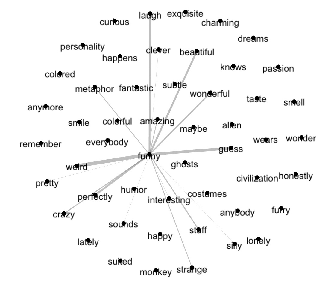

Top PageRank word - 'decrease':

display(foaf2dot(graphInsight2,"decrease"))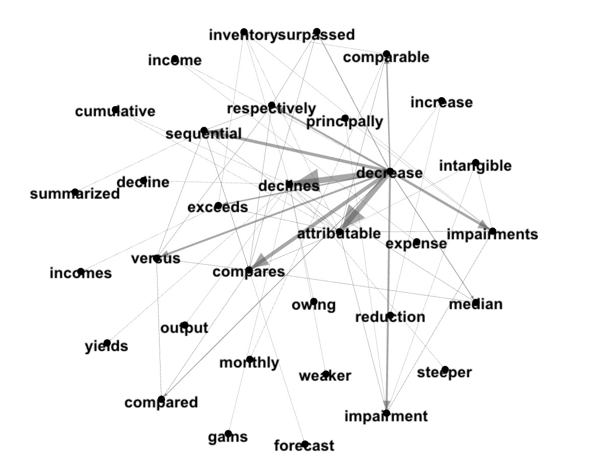

Top PageRank word - 'integrated':

display(foaf2dot(graphInsight2,"integrated"))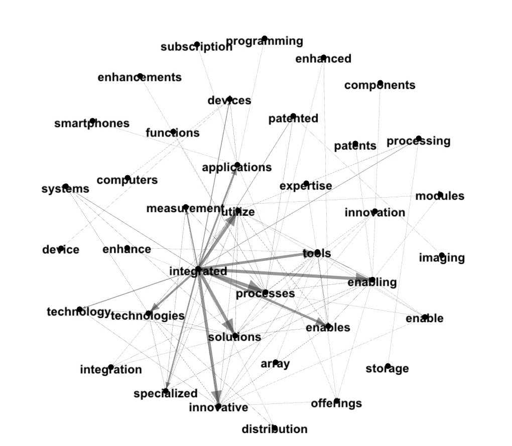

Top PageRank word - 'symptoms':

display(foaf2dot(graphInsight2,"symptoms"))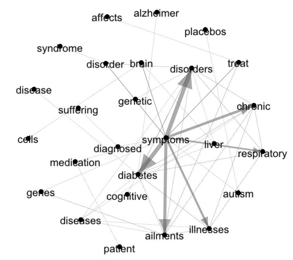

Top PageRank word - 'emory':

display(foaf2dot(graphInsight2,"emory"))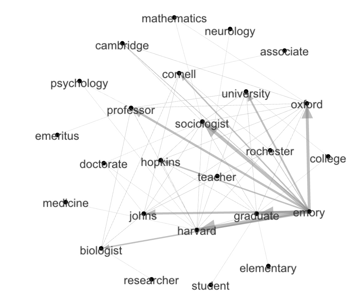

Next Post - Associations and Deep Learning

In the next post we will deeper look at deep learning for data associations.