From Unsupervised CNN Deep Learning Classification to Vector Similarity Metrics
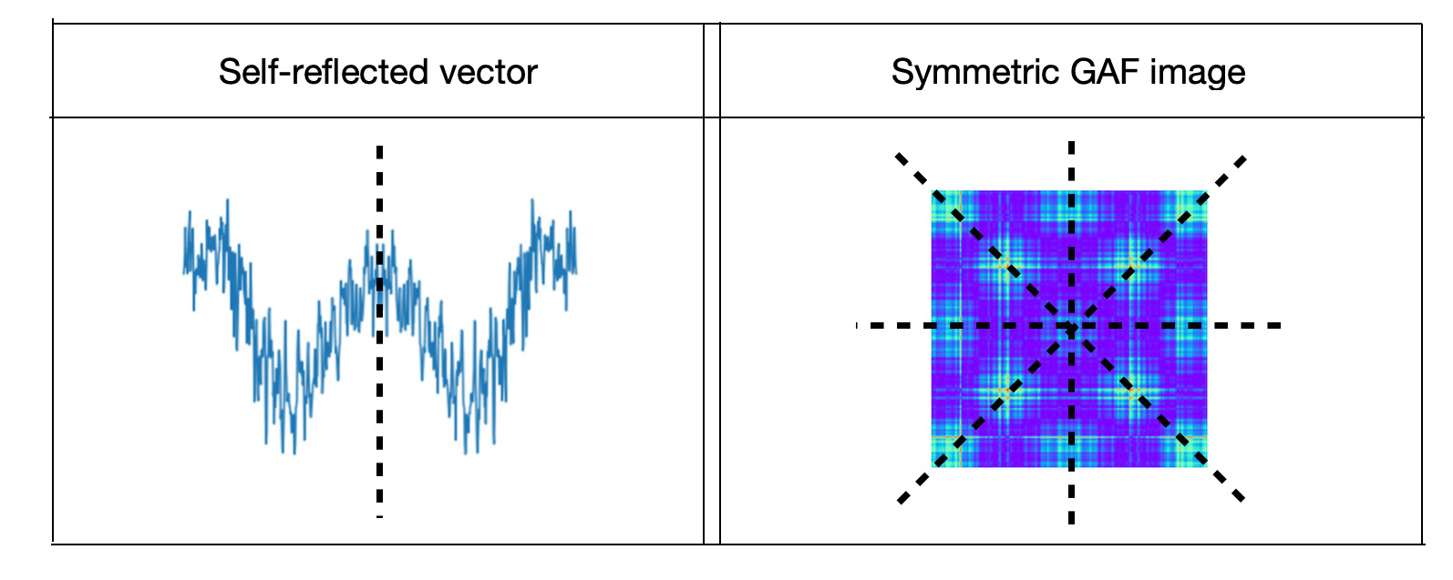
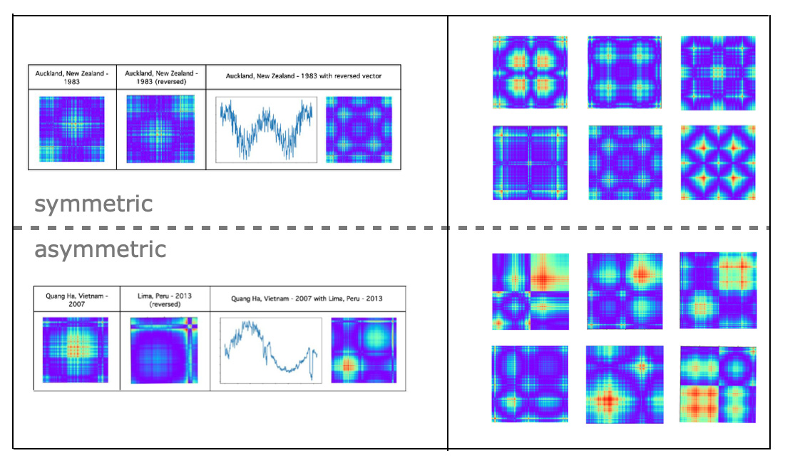
Vector similarity measures on large amounts of high-dimensional data has become essential in solving many machine learning problems such as classification, clustering or information retrieval. Traditional methods of vector similarity calculations are cosine similarities or dot products. In this post we propose a new method based on transforming vectors to images, classifying pairwise images and getting metric as model probability. For image classification we rely on outstanding success of Convolutional Neural Network image classification that in the last few years influenced application of this technique to extensive variety of objects. Our method takes advantages of CNN transfer learning image classification. To build a model for symmetry metrics, we concatenate vector pairs by reversing right vectors. If vectors are very similar the joint vectors will look like mirror vectors. Joint vectors will be transformed to GAF images that proved to get higher accuracy metrics for image classification than plot pictures of joint vectors.To distinguish between similar and dissimilar vector pairs we will generate training data as 'same' and 'different' classes. For the 'same' class we will generate self-reflected, mirror vectors and for 'different' class we will generate joint vectors as a random combination of non-equal pairs. Mirror vectors of the 'same' class transformed to GAF images represent symmetric images and GAF images of the 'different' class - asymmetric images. CNN image classification model is trained to distinguish between symmetric and asymmetric images. Similarity metric of this model is a probability for joint vectors converted to GAF image to get into the 'same' class.
In this post we will compare effectiveness of symmetry metrics and cosine similarity metrics for climate data analysis scenarios.
Introduction
Vector similarity measures on large amounts of high-dimensional data has become essential for solving many machine learning problems such as classification, clustering or information retrieval.
In the previous post "Unsupervised Deep Learning for Climate Data Analysis" we applied unsupervised machine learning model to categorize entity pairs to classes of similar and different pairs. This was done by transforming pairs of entities to pairwise vectors, transforming vectors to Gramian Angular Fields (GAF) images and classifying images by CNN transfer learning. That model allowed us to indicate metrics of GAF images visual similarity to symmetric or asymmetric classes.
In this post we will show how that model can be used to get 'same' probability metric for measuring similarities or dissimilarities between vectors. We will compare effectiveness of these metrics with effectiveness of cosine similarities.
In the previous post for experiments we selected climate data. In particular, we indicated when the model in not very reliable and illustrated several model reliable scenarios. Those reliable scenarios we will use in this post.
Unsupervised classification method that we introduced in "Unsupervised Deep Learning for Climate Data Analysis" to determine whether two vectors are similar or not to each other, we followed the steps:
- Created reflected pairwise vectors by concatenating pairs of vectors
- Transformed pairwise vectors to GAF images
- Train CNN transfer learning for image classification
Methods
In our previous post we introduced a novel unsupervised time series classification model. This model is embedding entities to vectors and combining entity pairs to pairwise vectors. Pairwise vectors are transformed to Gramian Angular Fields (GAF) images and GAF images are classified to symmetric or asymmetric classes using transfer learning CNN image classification. We examined how this model works for entity pairs with two-way and one-way relationships and indicated that it is not reliable for classification of entity pairs with two-way relationships.
Data Preparation
For data processing, model training and interpreting the results we will use the following steps:- Create pairs of pairwise vectors: self-reflected, mirror vectors for ’same’ class and concatenated different vectors for ’different’ class
- Transform joint vectors to GAF images for image classification
- Train CNN image classification on transfer learning to distinguish between symmetric and asymmetric images
- Get similarity metrics based on interpretation of trained model results
Transform Vectors to Images
As a method of vector to image translation we used Gramian Angular Field (GAF) - a polar coordinate transformation based techniques. We learned this technique in fast.ai 'Practical Deep Learning for Coders' class and fast.ai forum 'Time series/ sequential data' study group.
Training of Unsupervised Vector Classification Model
For this study we used fast.ai CNN transfer learning image classification. To deal with comparatively small set of training data, instead of training the model from scratch, we followed ResNet-50 transfer learning: loaded the results of model trained on images from the ImageNet database and fine tuned it with data of interest. Python code for transforming vectors to GAF images and fine tuning ResNet-50 is described in fast.ai forum.
Use Results of Trained Models
To calculate how similar are vectors to each other we will combine them as joint vectors and transform to GAF images. Then we will run GAF images through trained image classification model and use probabilities of getting to the ’same’ class as symmetry metrics. To predict vector similarities based on the trained model, we will use fast.ai function 'learn.predict'.Experiments
Climate Data
As a data source we will use climate data from Kaggle data sets: "Temperature History of 1000 cities 1980 to 2020" - daily temperature from 1980 to 2020 years for 1000 most populous cities in the world. In our previous posts we described the process of data preparation for pairwise vector method, model training and interpretation techniques are described in details in another post of our technical blog. In our post we proved the hypothesis that pairwise vector classification model is not reliable to predict similarity of pairs with two-way relationships. This hypothesis is based on the fact that GAF images being based on polar coordinates might generate inconsistent results for turned around entity pairs. In this post we will use two data sets that in the previous post we used as similarity prediction scenarios for pairs with one-way relationships. First, we will select daily temperature data for cities located in Western Europe, find a city located in the center of these cities and compare center city temperatures with other cities for years 2008 and 2016. For these combinations we will compare symmetry metrics, cosine similarities and distances between the cities. Second, we will calculate average vector of all yearly temperatures vectors for cities in Western Europe and compare it with yearly temperature vectors for all cities.Compare {City, Year} Temperature Vectors with Central City
The dataset for the first scenario consists of daily temperature time series for years 2008 and 2016 for cities in the contitental part of Western Europe. We selected 66 highly populous cities from the following countries:countryList=['Belgium', 'Germany', 'France','Austria','Netherlands','Switzerland',
'Spain','Italy','Denmark','Finland','Greece','Italy','Monaco',
'Netherlands','Norway','Portugal','Sweden','Switzerland']- To calculate symmetry metrics we will use the model trained on the whole climate data set for 1000 cities and years 1980 - 2019.
- For each city from our list we will create pairwise {City, Stuttgart} vectors for the years 2008 and 2016.
- Pairwise vectors will be transformed to GAF images and based on the trained model we will calculate probability of symmetric, i.e. 'same' class.
- We will calculate cosines between cities and Stuttgart daily temperature time series to compare metrics with cosine similarities.
- We will compare symmetry metrics and cosine similarities with distances between cities.
Training Model
Time series classification model training was done on fast.ai transfer learning method. For training data we used full data set about daily temperature for 1980 to 2020 years from 1000 most populous cities in the world. We created classes of symmetric images and asymmetric GAF images as:- For the ’same’ or 'symmetric' class we combined vectors with themselves reversing right side vectors.
- For the ’different’ or 'asymmetric' class we combined random pairs of vectors with temperatures of different years and different cities with reversed right vectors.
 To estimate the results we calculated accuracy metrics as the proportion of the total number of predictions that were correct. The training model accuracy metric was about 96.5 percent.
Symmetry Metrics based on Results of Trained Models
To calculate symmetry metrics for Western Europe city list we created pairwise vectors by concatenating temperature vector pairs {City, Stuttgart} for the years 2008 and 2016 and transforming joint vectors to GAF images. Then we ran GAF images through the trained image classification model and used probabilities of getting to the ’same’ class as symmetry metrics. To predict vector similarities based on the trained model, we used fast.ai function 'learn.predict':PATH_IMG='/content/drive/My Drive/city2/img4'
data = ImageDataBunch.from_folder(PATH_IMG, train=".", valid_pct=0.23,size=200)
learn = learner.cnn_learner(data2, models.resnet34, metrics=error_rate)
learn.load('stage-1a')Cosine Similarities
To compare with symmetry metrics we calculated cosine similarities between Stuttgart and other city daily temperatures for 2008 and 2016. For cosine similarities we used the following functions:import torch
def pytorch_cos_sim(a: Tensor, b: Tensor):
return cos_sim(a, b)
def cos_sim(a: Tensor, b: Tensor):
if not isinstance(a, torch.Tensor):
a = torch.tensor(a)
if not isinstance(b, torch.Tensor):
b = torch.tensor(b)
if len(a.shape) == 1:
a = a.unsqueeze(0)
if len(b.shape) == 1:
b = b.unsqueeze(0)
a_norm = torch.nn.functional.normalize(a, p=2, dim=1)
b_norm = torch.nn.functional.normalize(b, p=2, dim=1)
return torch.mm(a_norm, b_norm.transpose(0, 1))Distances Between City Pairs
To analyze symmetry metrics and cosine similarities we compared these metrics with distances between the cities. Here are functions to calculate the distance in kilometers by geographic coordinates:from math import sin, cos, sqrt, atan2, radians
def dist(lat1,lon1,lat2,lon2):
rlat1 = radians(float(lat1))
rlon1 = radians(float(lon1))
rlat2 = radians(float(lat2))
rlon2 = radians(float(lon2))
dlon = rlon2 - rlon1
dlat = rlat2 - rlat1
a = sin(dlat / 2)**2 + cos(rlat1) * cos(rlat2) * sin(dlon / 2)**2
c = 2 * atan2(sqrt(a), sqrt(1 - a))
R=6371.0
return R * cdef cityDist(city1,country1,city2,country2):
lat1=cityMetadata[(cityMetadata['city_ascii']==city1)
& (cityMetadata['country']==country1)]['lat']
lat2=cityMetadata[(cityMetadata['city_ascii']==city2)
& (cityMetadata['country']==country2)]['lat']
lon1=cityMetadata[(cityMetadata['city_ascii']==city1)
& (cityMetadata['country']==country1)]['lng']
lon2=cityMetadata[(cityMetadata['city_ascii']==city2)
& (cityMetadata['country']==country2)]['lng']
return dist(lat1,lon1,lat2,lon2)
Compare Symmetry Metrics and Cosine Similarities with Distances between Cities
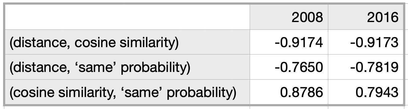
As expected, for both years, cities located close to Stuttgart have high cosine similarities and high probability of getting into the 'same' class by symmetry metrics. Here are correlation coefficients between distances and metrics for years 2008 and 2016:
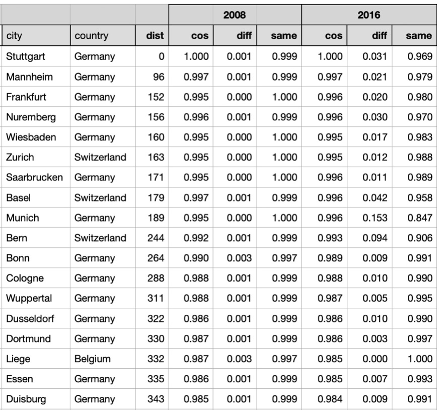
For most cities located far from Stuttgart daily temperature vectors have higher probabilities and lower cosine similarities than nearby cities. However by looking at symmetry metrics we can see that some cities located far from Stuttgart have rather similar daily temperature vectors. For example, daily weather in Oslo was similar to daily weather in Stuttgart with probability 0.942 in 2008 and with probability 0.498 in 2016.
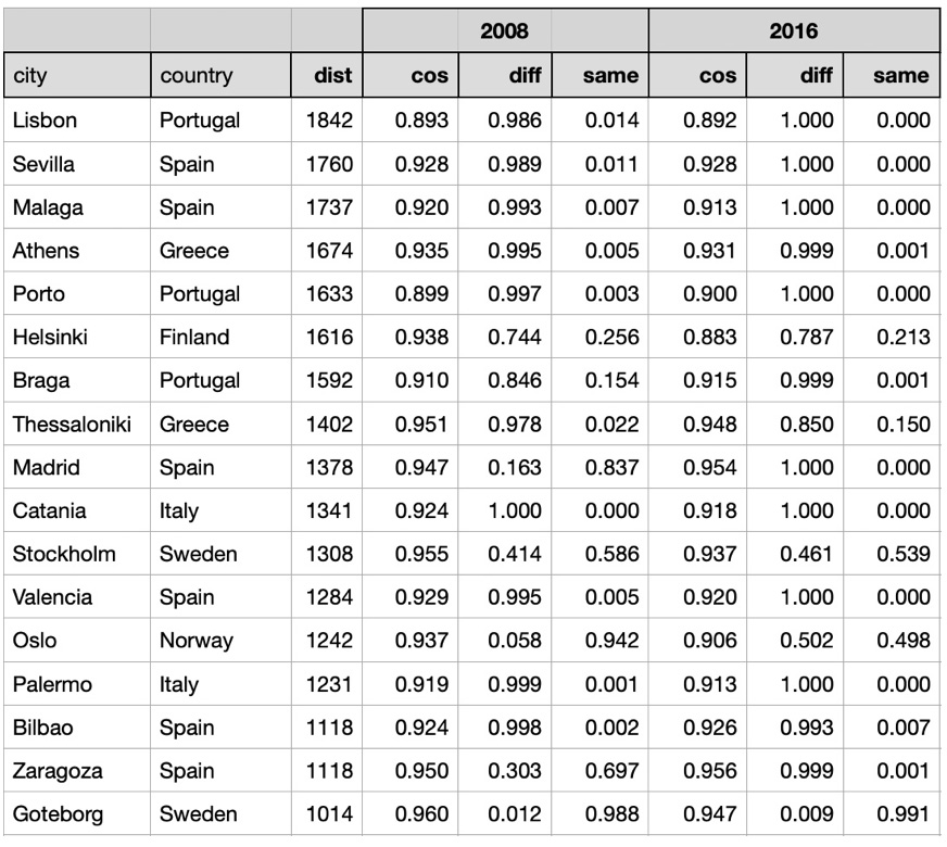 So for both years cities located close to Stuttgart had high cosine similarities and high probability of similar temperature vectors and cities located far from Stuttgart had low cosine similarities and low probabilities of similar temperature vectors.
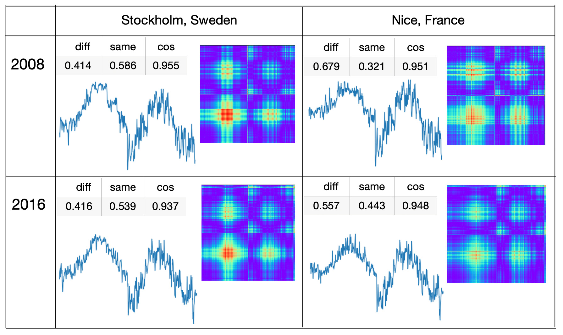
Not so easy was to predict which cities had similarities with Stuttgart temperatures on the border between ’different’ and ’same’. Here are two cities that in both years 2008 and 2016 have symmetry metrics close to 0.5. In the figure we also show cosine similarity metrics that don't look usefull to find {city, year} time series that are on the border between ’different’ and ’same’ classes.
So for both years cities located close to Stuttgart had high cosine similarities and high probability of similar temperature vectors and cities located far from Stuttgart had low cosine similarities and low probabilities of similar temperature vectors.
Not so easy was to predict which cities had similarities with Stuttgart temperatures on the border between ’different’ and ’same’. Here are two cities that in both years 2008 and 2016 have symmetry metrics close to 0.5. In the figure we also show cosine similarity metrics that don't look usefull to find {city, year} time series that are on the border between ’different’ and ’same’ classes.
ABS(0.5 - same probability for 2008) * ABS(0.5 - same probability for 2016)
 Here you can see that symmetry metrics help to find 'on the border' {city, year} time series and cosine similarity metrics are not helpfull to find such time series.
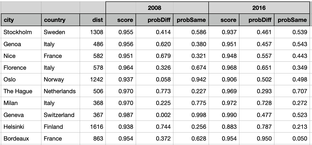
Compare {City, Year} Temperature Vectors with Average of All Yearly Temperatures
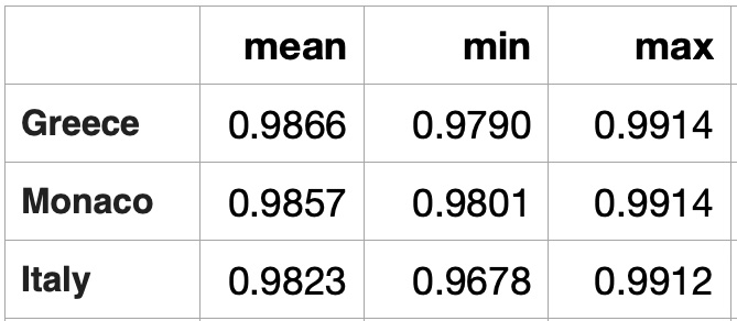
For another scenario we calculated average vector for 2640 daily temperature time series - for years from 1980 to 2019 for 66 Western Europen cities and compared this vector it with yearly temperature vectors for all cities. Average of 2460 city-year temperature vectors provides a very smooth line, we did not expect many similar city-year temperature vectors. With symmetry metrics we found that most of cities with high similarities to a smooth line are located on Mediterranean Sea not far from each other. Here is a clockwise city list: Marseille (France), Nice (France), Monaco (Monaco), Genoa (Italy), Rome (Italy), Naples (Italy), and Salerno (Italy):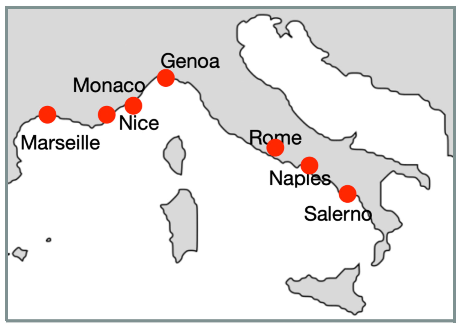 Countries with daily temperature statistically similar to the average of average.
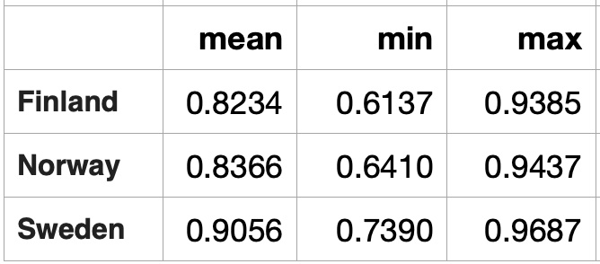
 Countries with daily temperature statistically sfar from the average of average.
Conclusion
In this post we introduced symmetry metrics for high dimensional vector similarity based on unsupervised pairwise vector classification model. This model is implemented through transforming joint vectors to GAF images and classifying images as symmetric or asymmetric. Symmetry metric is defined as a probability of GAF image ran through trained model and get to the ’same’, i.e. 'symmetric' class. In this post we demonstrated how the symmetry metric can be used to measure differences between vectors instead of measuring them through traditional cosine similarity approach. We examined effectiveness of symmetry metrics for entity pair analysis and compared the results with cosine similarity metrics.Broader Impact and Future Work
In the future we are planning to experiment with symmetry metrics for different aspects.- So far our research about symmetry metrics was limited to time series data mining. In addition to time series, symmetry metrics can be applied to a variety of embeddable entity pairs such as words, documents, images, videos, etc. For example, symmetry metrics can be used for unsupervised outlier detection in finding stock price that are very different from average stock prices.
- Potentially pairwise vectors model trained on symmetric and asymmetric GAF images can be trained on some data domain and used for other data domains. For example, we are planning to evaluate how the model trained on time series data can be used for word similarity classification.
- Furthermore, as direct graphs can be built through symmetry metrics, we are planning to experiment on using these metrics for Graph Neural Network research.