Unified Knowledge Graph for Artists and Paintings
Think of this project as one map of the art world, where artists and paintings are dots and their relationships form the lines between them. We turn biographies and images into a single unified knowledge graph, then use Graph AI to see which artists and works are close, far, or unexpectedly linked. Instead of scrolling through lists, you can explore art as a connected network and discover relationships you wouldn’t notice from text or images alone. The same pattern extends far beyond art: this pipeline can fuse text, images, time series, and other data into a unified knowledge graph in any domain, keeping everything analyzable with one Graph AI workflow.
Conference & Publication
This work was presented at CVIT 2025 in Florence, Italy, on June 20, 2025, and published as: Romanova, A. (2025). “Rewiring Multi-Modal Knowledge Graphs with GNN Link Prediction: Insights from Art History.” doi: 10.1117/12.3078062.
Introduction: Knowledge Graphs Exploration
Art and artists are deeply connected, reflecting creativity, culture, and history. Graphs provide a powerful way to explore these relationships by representing artists, artworks, and movements as nodes, and their connections as edges. This helps us uncover patterns, find hidden links, and better understand the evolution of art. With advanced tools like Graph Neural Networks (GNNs), we can predict new connections, group related ideas, and gain even deeper insights into the art world.Building on Our Previous Research
The first study, titled "Building Knowledge Graph in Spark without SPARQL", was presented at the DEXA 2020 online conference. It explored non-traditional methods for constructing and analyzing knowledge graphs, moving beyond SPARQL-based semantic web approaches. The study demonstrated how the Spark GraphFrames library could be leveraged to efficiently build and mine knowledge graphs. Focusing on modern art artists, it highlighted the versatility and scalability of knowledge graph techniques.
For more details, visit: Building Knowledge Graph in Spark without SPARQL
Reference: Romanova, A. (2020). Building knowledge graph in spark without SPARQL. CCIS, vol. 1285, pp 96–102.
The second study was presented at ICAART 2023: 22-24 February, 2023 in Lisbon. It focused on methods for rewiring knowledge graphs to uncover hidden relationships between nodes using GNN link prediction models. The experiments analyzed semantic similarities and dissimilarities between the biographies of modern art artists by utilizing Wikipedia articles. A traditional method used the full text of articles and cosine similarities between re-embedded nodes, while a novel method examined the distribution of co-located words within and across articles. Output vectors from the GNN link prediction model were aggregated by artist, and link predictions were calculated based on cosine similarities.
The study highlighted the importance of both highly connected and highly disconnected node pairs in graph mining. Disconnected pairs offered unique insights, revealing the knowledge graph's overall coverage and serving as indicators for validating community detection. Additionally, the study demonstrated practical applications for rewired knowledge graphs in recommender systems. High-similarity node pairs suggested related artists or movements, while high-dissimilarity pairs encouraged users to explore contrasting art movements, enhancing the diversity of recommendations.
For more details, visit: Rewiring Knowledge Graphs by Graph Neural Network Link Predictions
Reference: Romanova, A. Rewiring Knowledge Graphs by Graph Neural Network Link Predictions. International Conference on Agents and Artificial Intelligence (2023). doi:10.5220/0011664400003393.
This Study
The dataset, 'Best Artworks of All Time', was taken from Kaggle. It features information and artwork images from 50 of the most influential artists in history. The dataset includes detailed artist metadata sourced from Wikipedia, as well as a collection of high-resolution images scraped from artchallenge.ru. This study focuses on the Construction of a Unified Knowledge Graph to analyze the relationships between artists and their works. Starting with raw data comprising artist biographies and painting images, two separate graphs are created: an Artist Graph and a Painting Graph. Textual data from artist biographies is transformed into vectors using Large Language Models (LLMs), while visual data from painting images is processed into vectors using Convolutional Neural Networks (CNNs). These initial embeddings are further refined through Graph Neural Networks (GNNs) to produce consistent, high-quality representations for the nodes in both graphs. The final step involves combining the Artist Graph and Painting Graph into a single Unified Knowledge Graph, where links represent the connections between artists and their respective works. This integrated graph provides a robust framework for exploring the intricate relationships within the art world, enabling tasks such as classification, clustering, and link prediction.
Methods
Graph Construction for Artists
The process of constructing a graph to represent artist relationships begins with defining nodes for each artist and creating edges based on shared attributes such as genre and nationality.
Each artist is represented as a node in the graph, with attributes like the artist's index and name. To capture relationships:
- Genre-Based Edges: Edges are added between all pairs of artists who share the same genre, reflecting thematic or stylistic connections.
- Nationality-Based Edges: Edges are created between artists who share the same nationality, representing cultural or geographical ties.
To enable analysis, the graph’s edges are converted into a DataFrame, organized with columns for source nodes, target nodes, and edge attributes. If the edge attributes are stored as dictionaries, these are expanded into individual columns for easier interpretation. The resulting DataFrame is reviewed to confirm its accuracy and structure.
Transforming Text to Vectors for Node Features
Artist biographies are transformed into vector embeddings to enrich the graph with semantic information. Using the Hugging Face 'all-MiniLM-L6-v2' model, the text is encoded into a 384-dimensional vector space, producing a tensor of size [50, 384], where each row represents an artist.
These embeddings are assigned as node features in the graph using the ndata['feat'] attribute. This enables:
- Using vectors as input for GNN link prediction models.
- Generating additional graph edges by calculating a cosine similarity matrix and selecting highly connected vector pairs.
This approach provides a robust foundation for graph-based analysis, capturing both semantic relationships and potential hidden connections between artists.
Run GNN Link Prediction Model
As Graph Neural Networks link prediction we used a model from Deep Graph Library (DGL). The model is built on two GrapgSAGE layers and computes node representations by averaging neighbor information. We used the code provided by DGL tutorial DGL Link Prediction using Graph Neural Networks.
The results of this code are embedded nodes that can be used for further analysis such as node classification, k-means clustering, link prediction and so on. In this study we used it for link prediction by estimating cosine similarities between embedded nodes.
Building the Painting Graph
To construct a graph representing paintings, artwork files are processed to link paintings to their respective artists and prepare the data for graph creation. Each painting is assigned a unique File Index, and artist names extracted from file names are mapped to their corresponding Artist Index using artists_df. This information—File Name, Artist Name, File Index, and Artist Index—is combined into a structured DataFrame.
The Painting Graph is created where nodes represent paintings and edges connect paintings by the same artist. Using NetworkX, nodes are added with their File Index as identifiers and File Name as attributes. Edges are added between paintings that share the same Artist Index, capturing relationships based on shared creators.
Image Features for Node Embeddings
Painting images are processed to generate visual embeddings using a pre-trained CNN, such as ResNet. Images are resized, normalized, and passed through the model to extract high-dimensional feature vectors. These embeddings are stored as node features, enriching the graph with visual content for machine learning tasks.
Transforming the Painting Graph to DGL Format
The Painting Graph is converted into DGL format to facilitate efficient processing and modeling using DGL's graph-based machine learning tools. The edges from painting_graph_edges are transformed into a PyTorch tensor, defining the graph's structure. Self-loops are added to ensure each node is connected to itself, which can enhance the performance of GNN models.
Image feature vectors, previously saved and loaded from storage, are assigned as node features in the graph. These embeddings are converted into a PyTorch tensor and set using the ndata['feat'] attribute, enriching the graph with meaningful visual data for each painting node.
GNN Link Prediction Model Training for the Painting Graph
The GNN model is trained for link prediction on the Painting Graph using the constructed graph and its visual embeddings. Similar to the Artist Graph, the training process involves predicting links by leveraging the node features, allowing the model to identify relationships between paintings based on shared visual or contextual patterns. This tailored approach reveals hidden connections and enhances the understanding of painting relationships within the graph.
Unified Knowledge Graph
To analyze relationships between artists and their works, we created a Unified Knowledge Graph by combining the Artist graph and Painting graph. This integration enables consistent multi-modal data embedding and analysis.
Artist biographies were transformed into 384-dimensional vectors using a transformer model, then reduced to 128-dimensional embeddings through GNN link prediction. Paintings were similarly represented as 2048-dimensional vectors using a pre-trained CNN model, which were also reduced to 128-dimensional embeddings.
To unify the graphs, unique indices ensured no overlap between artist and painting nodes, with artist nodes offset by 1000. Painting file names were processed to map each painting to its corresponding artist, and edges were added to represent these relationships.
The resulting Unified Knowledge Graph integrates artist and painting data into a single structure, providing a foundation for advanced graph-based analysis.
GNN Link Prediction Model for the Unified Graph
We applied the GNN Link Prediction model three times across different stages of the study:
1. Artist Graph: The model was used to process artist biographies, initially embedded as 384-dimensional vectors derived from text data. The GNN Link Prediction model reduced these embeddings to a consistent size of 128 dimensions, capturing semantic relationships between artists effectively.
2. Painting Graph: For paintings, visual features extracted via a CNN model were initially represented as 2048-dimensional vectors. The GNN Link Prediction model was applied to reduce these high-dimensional embeddings to 128 dimensions, emphasizing meaningful stylistic or thematic connections between paintings.
3. Unified Knowledge Graph: After merging the Artist and Painting graphs into a single structure, the GNN Link Prediction model was run again on the unified graph. This step refined the node embeddings, ensuring consistent 128-dimensional representations across all nodes while integrating multi-modal relationships between artists and their works.
By running the model at each stage, we achieved consistent embeddings that facilitate advanced graph-based analysis, uncovering complex patterns and relationships within the unified framework.
Experiments
Data Source Analysis
As data source we used text data from kaggle.com: 'Best Artworks of All Time'.Metadata Overview
This dataset provides the following key files:
-
artists.csv:- Contains metadata for 50 influential artists, including:
- Name, Genre, Nationality, Biography, and Years (lifespan or active period).
-
resized.zip:- A collection of resized artwork images, optimized for faster processing and reduced storage.
- Ideal for machine learning workflows requiring efficient model training and testing.
These files provide a compact yet comprehensive resource for analyzing and classifying artworks.
Raw Data Processing
The code loads the artist metadata from a CSV file, selects relevant columns (name, genre, nationality, bio, years), sorts the data alphabetically by name, resets the index, and assigns a sequential artistIndex based on the new order.artists = pd.read_csv("/content/drive/My Drive/Art/artists.csv")
artists_dff = artists[['name', 'genre', 'nationality','bio', 'years']]
artists_df= artists_dff.sort_values('name').reset_index(drop=True)
artists_df['artistIndex'] = artists_df.indexSplit the standardized 'years' column into 'start_year' and 'end_year':
-
The
yearscolumn is cleaned to replace special characters (e.g., em-dash) with a hyphen and split intostart_yearandend_year. -
The
genrecolumn is exploded, creating separate rows for each genre associated with an artist, and the DataFrame is reset to includeartistIndex,name,start_year,end_year, andgenre. -
A new DataFrame,
artist2nationality, is created by splitting thenationalitycolumn into multiple entries, exploding it into separate rows, and resetting the index to includeartistIndex,name,start_year,end_year, andnationality.
artists_df['years'] = artists_df['years'].apply(lambda x: re.sub(r'[–—]', '-', x))
artists_df[['start_year', 'end_year']] = artists_df['years'].str.split(' - ', expand=True)
  .explode('genre')
  .reset_index(drop=True)[['artistIndex', 'name', 'start_year', 'end_year', 'genre']]
artist2nationality = artists_df.assign(nationality=artists_df['nationality'].str.split(',')) \
.explode('nationality')
.reset_index(drop=True)[['artistIndex', 'name', 'start_year', 'end_year', 'nationality']]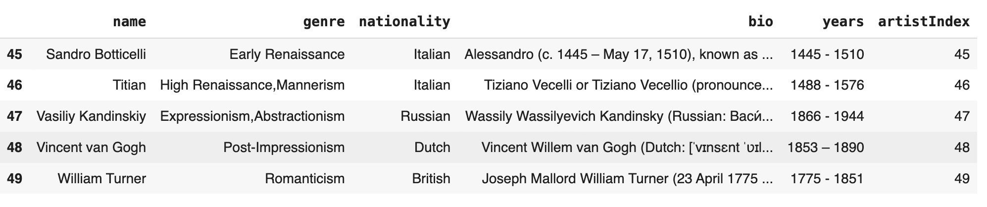
Artist Graph
Building Graph on Artists
To construct a graph where nodes represent artists and edges are created based on shared attributes, follow these steps:
-
Create nodes: Add a node for each artist using their
artistIndexandname. - Create genre-based edges: For each genre, add edges between all pairs of artists who share that genre.
- Create nationality-based edges: Similarly, for each nationality, add edges between all pairs of artists who share that nationality.
import networkx as nx
G = nx.Graph()
for _, row in artist2genre.iterrows():
    G.add_node(row['artistIndex'], name=row['name'])# !pip install torch
for genre, group in artist2genre.groupby('genre'):
    artist_indices = group['artistIndex'].tolist()
    for i in range(len(artist_indices)):
        for j in range(i + 1, len(artist_indices)):
            G.add_edge(artist_indices[i], artist_indices[j], genre=genre)
for nationality, group in artist2nationality.groupby('nationality'):
    artist_indices = group['artistIndex'].tolist()
    for i in range(len(artist_indices)):
        for j in range(i + 1, len(artist_indices)):
            G.add_edge(artist_indices[i], artist_indices[j], nationality=nationality)
print(f"Number of nodes: {G.number_of_nodes()}")
print(f"Number of edges: {G.number_of_edges()}")
print(f"Average degree: {nx.density(G) * (G.number_of_nodes() - 1)}")
Number of nodes: 50
Number of edges: 218
Average degree: 8.72
The following steps describe how to convert graph edges into a DataFrame for analysis:
- Convert edges to a DataFrame: Extract the edges from the graph
Gand organize them into a DataFrame with columns for source nodes, target nodes, and edge attributes. - Expand edge attributes: If the edge attributes are stored as dictionaries, expand these into separate columns to make them more accessible.
- Display the edges DataFrame: View the resulting DataFrame to verify its structure and content.
The Python code snippet below demonstrates these steps:
import pandas as pd
edges_df = pd.DataFrame(list(G.edges(data=True)), columns=['Source', 'Target', 'Attributes'])
if not edges_df.empty and isinstance(edges_df['Attributes'].iloc[0], dict):
    attributes_df = edges_df['Attributes'].apply(pd.Series)
edges_df = pd.concat([edges_df.drop(columns=['Attributes']), attributes_df], axis=1)import dgl
import dgl.nn as dglnn
import dgl.data
from dgl.data import DGLDataset
import torch
import torch.nn as nn
import torch.nn.functional as F
import itertools
unpickEdges=edges_df
edge_index=torch.tensor(unpickEdges[['Source','Target']].T.values)
u,v=edge_index[0],edge_index[1]
g=dgl.graph((u,v))
g=dgl.add_self_loop(g)
g
Graph(num_nodes=50, num_edges=268,
ndata_schemes={}
edata_schemes={})Transform Text to Vectors
This section describes how text data, specifically the artist biographies, is transformed into vector embeddings to be used as node features in a graph. We utilized the 'all-MiniLM-L6-v2' model from Hugging Face for this purpose, which generates high-quality sentence embeddings.
-
Model Selection: The
'all-MiniLM-L6-v2'model, a lightweight yet powerful transformer, was used for efficient text-to-vector translation. -
Embedding Creation: Artist biographies from the DataFrame are encoded into a tensor of size
[50, 384], where each row represents a 384-dimensional vector for an artist. -
Assigning Features: These embeddings are assigned as node features to the graph using the
ndata['feat']attribute.
model = SentenceTransformer('all-MiniLM-L6-v2')
node_embeddings = modelST.encode(artists_df['bio'],convert_to_tensor=True)
node_embeddings = node_embeddings.to(torch.device('cpu'))
gNew.ndata['feat'] = node_embeddings
node_embeddings.shape
torch.Size([50, 384])g
Graph(num_nodes=50, num_edges=268,
ndata_schemes={'feat': Scheme(shape=(384,), dtype=torch.float32)}
edata_schemes={})GNN Link Prediction Model Training
This subsection describes the process of training a GNN link prediction model, using code adapted from the DGL library. The focus is on leveraging the built-in functionalities for implementing and training GNN-based link prediction tasks.
The training pipeline includes constructing positive and negative edge graphs for the training and testing phases, defining the GNN architecture, and training the model using standard techniques. The training concludes with an evaluation of the model's performance using the AUC (Area Under the Curve) metric.
u, v = g.edges()
eids = np.arange(g.number_of_edges())
eids = np.random.permutation(eids)
test_size = int(len(eids) * 0.1)
train_size = g.number_of_edges() - test_size
test_pos_u, test_pos_v = u[eids[:test_size]], v[eids[:test_size]]
train_pos_u, train_pos_v = u[eids[test_size:]], v[eids[test_size:]]
adj = sp.coo_matrix((np.ones(len(u)), (u.numpy(), v.numpy())))
adj_neg = 1 - adj.todense() - np.eye(g.number_of_nodes())
neg_u, neg_v = np.where(adj_neg != 0)
neg_eids = np.random.choice(len(neg_u), g.number_of_edges())
test_neg_u, test_neg_v = neg_u[neg_eids[:test_size]], neg_v[neg_eids[:test_size]]
train_neg_u, train_neg_v = neg_u[neg_eids[test_size:]], neg_v[neg_eids[test_size:]]
train_g = dgl.remove_edges(g, eids[:test_size])
from dgl.nn import SAGEConv
class GraphSAGE(nn.Module):
def __init__(self, in_feats, h_feats):
super(GraphSAGE, self).__init__()
self.conv1 = SAGEConv(in_feats, h_feats, 'mean')
self.conv2 = SAGEConv(h_feats, h_feats, 'mean')
def forward(self, g, in_feat):
h = self.conv1(g, in_feat)
h = F.relu(h)
h = self.conv2(g, h)
return himport dgl.function as fn
train_pos_g = dgl.graph((train_pos_u, train_pos_v), num_nodes=g.number_of_nodes())
train_neg_g = dgl.graph((train_neg_u, train_neg_v), num_nodes=g.number_of_nodes())
test_pos_g = dgl.graph((test_pos_u, test_pos_v), num_nodes=g.number_of_nodes())
test_neg_g = dgl.graph((test_neg_u, test_neg_v), num_nodes=g.number_of_nodes())
class DotPredictor(nn.Module):
def forward(self, g, h):
with g.local_scope():
g.ndata['h'] = h
g.apply_edges(fn.u_dot_v('h', 'h', 'score'))
return g.edata['score'][:, 0]class MLPPredictor(nn.Module):
def __init__(self, h_feats):
super().__init__()
self.W1 = nn.Linear(h_feats * 2, h_feats)
self.W2 = nn.Linear(h_feats, 1)
def apply_edges(self, edges):
h = torch.cat([edges.src['h'], edges.dst['h']], 1)
return {'score': self.W2(F.relu(self.W1(h))).squeeze(1)}
def forward(self, g, h):
with g.local_scope():
g.ndata['h'] = h
g.apply_edges(self.apply_edges)
return g.edata['score']model = GraphSAGE(train_g.ndata['feat'].shape[1], 128)
pred = MLPPredictor(128)
def compute_loss(pos_score, neg_score):
scores = torch.cat([pos_score, neg_score])
labels = torch.cat([torch.ones(pos_score.shape[0]), torch.zeros(neg_score.shape[0])])
return F.binary_cross_entropy_with_logits(scores, labels)
def compute_auc(pos_score, neg_score):
scores = torch.cat([pos_score, neg_score]).numpy()
labels = torch.cat(
[torch.ones(pos_score.shape[0]), torch.zeros(neg_score.shape[0])]).numpy()
return roc_auc_score(labels, scores)
optimizer = torch.optim.Adam(itertools.chain(model.parameters(), pred.parameters()), lr=0.01)all_logits = []
for e in range(100):
h = model(train_g, train_g.ndata['feat'].float())
pos_score = pred(train_pos_g, h)
neg_score = pred(train_neg_g, h)
loss = compute_loss(pos_score, neg_score)
optimizer.zero_grad()
loss.backward()
optimizer.step()
if e % 5 == 0:
print('In epoch {}, loss: {}'.format(e, loss))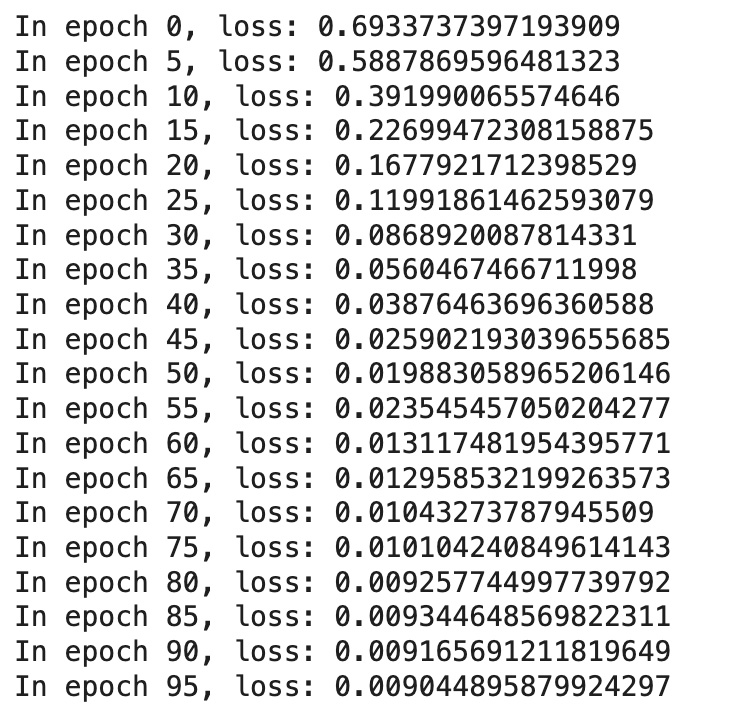 Final evaluation:
from sklearn.metrics import roc_auc_score
with torch.no_grad():
    pos_score = pred(test_pos_g, h)
    neg_score = pred(test_neg_g, h)
    print('AUC', compute_auc(pos_score, neg_score))
AUC 0.9171597633136095
To ensure the embedded vectors are preserved and accessible across sessions, they are saved to Google Drive as PyTorch tensors. This allows seamless reuse without recomputing the embeddings, saving time and computational resources.
import torch
torch.save(h, '/content/drive/My Drive/Art/artists_h.pt')
load_h = torch.load('/content/drive/My Drive/Art/artists_h.pt')
Paintings Graph
Create a Graph on Paintings
In this subsection, we process artwork files to build a DataFrame that links paintings to their respective artists and prepares data for graph construction.
The following steps outline the workflow:
-
Process files in the directory: Iterate through the files in the specified directory, extract the painting's file name, artist's name, and assign a unique
File Indexto each painting. -
Match artist names to indices: The artist names extracted from the file names are mapped to their corresponding
Artist Indexusing a sorted version of theartists_df. -
Create the paintings DataFrame: Combine the extracted file data, including
File Name,Artist Name,File Index, and the mappedArtist Index, into a structured DataFrame for further analysis and graph creation.
paintings_dir = '/content/drive/My Drive/Art/paintings/'
import os
import pandas as pd
file_data = []
file_index = 0
if os.path.exists(paintings_dir):
    for file in sorted(os.listdir(paintings_dir)):
        if os.path.isfile(os.path.join(paintings_dir, file)):
            artist_name = file.rsplit('_', 1)[0].replace('_', ' ')
            file_data.append((file, artist_name, file_index))
            file_index += 1
columns = ['File Name', 'Artist Name', 'File Index']
file_df = pd.DataFrame(file_data, columns=columns)
artists_sorted = artists_df.sort_values('name').reset_index(drop=True)
artist_name_to_index = {name: idx for idx, name in enumerate(artists_sorted['name'])}
file_df['Artist Index'] = file_df['Artist Name'].map(artist_name_to_index)
file_df.tail()
Initialize and Build the Painting Graph
This subsection describes the creation of a graph where nodes represent paintings, and edges connect paintings created by the same artist. The graph is then analyzed and converted to DGL format for use in machine learning tasks.
The following steps outline the workflow:
- Initialize the graph: Use NetworkX to create an undirected graph.
-
Add nodes with attributes: Each painting is added as a node, with its
File Indexas the identifier andFile Nameas a node attribute. -
Add edges: Paintings created by the same artist are connected. Edges are added between all pairs of paintings that share the same
Artist Index.
The Python code below demonstrates the implementation:
import networkx as nx
G = nx.Graph()
for _, row in file_df.iterrows():
    G.add_node(row['File Index'], file_name=row['File Name'])
artist_groups = file_df.groupby('Artist Index')['File Index'].apply(list)
for group in artist_groups:
    for i in range(len(group)):
        for j in range(i + 1, len(group)):
            G.add_edge(group[i], group[j])
print(f"Number of nodes: {G.number_of_nodes()}")
print(f"Number of edges: {G.number_of_edges()}")
print(f"Average degree: {nx.density(G) * (G.number_of_nodes() - 1)}")
Number of nodes: 1000
Number of edges: 9500
Average degree: 177.781nodes_data = [{'Node': n, **G2.nodes[n]} for n in G2.nodes]
nodes_df = pd.DataFrame(nodes_data)
nodes_df.to_csv('/content/drive/My Drive/Art/painting_graph_nodes.csv', index=False)edges_data = [{'Source': u, 'Target': v, **G2.edges[u, v]} for u, v in G2.edges]
edges_df = pd.DataFrame(edges_data)
edges_df.to_csv('/content/drive/My Drive/Art/painting_graph_edges.csv', index=False)Image Features for Node Embeddings
In this section, we use a pre-trained Convolutional Neural Network (CNN) to extract feature embeddings from the painting images. These features serve as node embeddings for the graph, enabling the model to capture meaningful visual patterns.
Workflow:
-
Image Preprocessing: Images are resized to
224x224pixels, converted to tensors, and normalized using standard ImageNet mean and standard deviation values. This ensures compatibility with the pre-trained CNN model. - Feature Extraction: Each preprocessed image is passed through the CNN (e.g., ResNet) to extract a high-dimensional feature vector. These vectors represent the visual content of the paintings.
- Embedding Storage: The extracted feature vector for each image is flattened, converted to a NumPy array, and stored in a dictionary with the file name as the key. This allows easy mapping between the image and its corresponding feature representation.
This process generates a rich set of visual embeddings that can be used as input features for graph-based learning tasks.
from torchvision import models, transforms
from PIL import Image
import torch
import os
transform = transforms.Compose([
    transforms.Resize((224, 224)),
    transforms.ToTensor(),
    transforms.Normalize(mean=[0.485, 0.456, 0.406], std=[0.229, 0.224, 0.225]),
])
image_vectors = {}
for file_name in file_names:
    img_path = os.path.join(paintings_dir, file_name)
    img = Image.open(img_path).convert('RGB')
    img_tensor = transform(img).unsqueeze(0)
    with torch.no_grad():
        features = model(img_tensor).flatten().numpy()
image_vectors[file_name] = featuresvectors_df = pd.DataFrame(image_vectors)
vectors_df.to_csv('/content/drive/My Drive/Art/image_vectors.csv', index=False)
loaded_image_vectors_df = pd.read_csv('/content/drive/My Drive/Art/image_vectors.csv')
loaded_image_vectors_df.shape
(2048, 1000)Transforming the Painting Graph to DGL Format
This subsection describes the process of transforming the painting graph into DGL format, including edge and node feature assignments. This transformation enables efficient processing and modeling using DGL's graph-based machine learning tools.
The previously saved image feature vectors are loaded from the CSV file stored on Google Driveimage_vectors = pd.read_csv("/content/drive/My Drive/Art/image_vectors.csv")
image_vectors.head()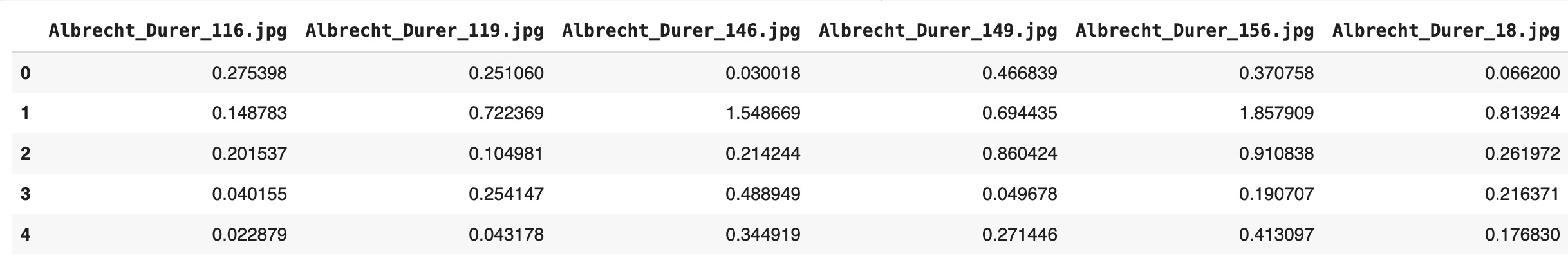
Workflow:
-
Create the DGL graph: The edges from
painting_graph_edgesare converted into a PyTorch tensor and used to define the graph structure. Self-loops are added to ensure every node has a connection to itself, which can enhance model performance. -
Assign node features: The image embeddings are transformed into a PyTorch tensor and assigned to the graph as node features using the
ndata['feat']attribute. This allows the graph to carry meaningful data for each node.
The following code demonstrates the transformation process:
unpickEdges=painting_graph_edges
edge_index=torch.tensor(unpickEdges[['Source','Target']].T.values)
u,v=edge_index[0],edge_index[1]
gPaintings=dgl.graph((u,v))
gPaintings=dgl.add_self_loop(gPaintings)
gPaintings
Graph(num_nodes=1000, num_edges=10500,
      ndata_schemes={}
edata_schemes={})image_vectors_T = image_vectors.T
image_vectors_T_df=pd.DataFrame(image_vectors_T).reset_index(drop=True)
import torch
image_vectors_tensor = torch.tensor(image_vectors_T_df.values, dtype=torch.float)
gPaintings.ndata['feat'] = image_vectors_tensor
gPaintings
Graph(num_nodes=1000, num_edges=10500,
ndata_schemes={'feat': Scheme(shape=(2048,), dtype=torch.float32)}
edata_schemes={})The resulting graph gPaintings includes 1000 nodes, 10,500 edges, and node features of shape (2048,). It is now ready for use in graph-based machine learning tasks.
GNN Link Prediction Model Training for the Painting Graph
In this subsection, we focus on training a GNN model for link prediction on the painting graph, utilizing the graph and node features constructed in the previous steps. This process is similar to the training conducted for the artist graph but specifically tailored to predict links between paintings based on their visual embeddings.- Forward pass: The node features (image embeddings) are passed through the GNN model to compute embeddings for each painting. Positive and negative edge scores are calculated using the model's prediction function.
- Loss computation: A loss function compares the predicted scores against the ground truth, guiding the model's optimization.
- Backward pass and optimization: Gradients are calculated with respect to the loss, and the optimizer updates the model's parameters to minimize the loss.
all_logits = []
for e in range(100):
    # forward
    h = model(train_g, train_g.ndata['feat'].float())
    pos_score = pred(train_pos_g, h)
    neg_score = pred(train_neg_g, h)
    loss = compute_loss(pos_score, neg_score)
    # backward
    optimizer.zero_grad()
    loss.backward()
    optimizer.step()
    if e % 5 == 0:
        print('In epoch {}, loss: {}'.format(e, loss))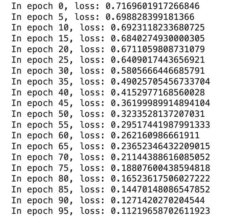
from sklearn.metrics import roc_auc_score
with torch.no_grad():
    pos_score = pred(test_pos_g, h)
    neg_score = pred(test_neg_g, h)
    print('AUC', compute_auc(pos_score, neg_score))
AUC 0.9827046611570248torch.save(h, '/content/drive/My Drive/Art/paintings_h.pt')
load_h = torch.load('/content/drive/My Drive/Art/paintings_h.pt')
load_h.shape
torch.Size([1000, 128])Unified Knowledge Graph
Combining Artist and Painting Graphs into a Unified Knowledge Graph
We started by constructing two separate graphs:
-
Artist Graph: Artist biographies were converted into vectors of size
384using a transformer model, followed by GNN link prediction, which transformed these embeddings into vectors of size128. -
Painting Graph: Paintings were represented as vectors of size
2048using a pre-trained CNN model, followed by GNN link prediction, which transformed these embeddings into vectors of size128.
Next Step: We will combine the Artist graph and Painting graph into a unified Knowledge Graph. This Knowledge Graph (suggested name: ArtKnowledgeGraph) will map painting nodes to their corresponding artist nodes. The node features for this unified graph will be represented by vectors of size 128, ensuring a consistent embedding space across all node types.
To create a unified Knowledge Graph, we need to ensure that nodes from both the Artist graph and the Painting graph have unique indices. This adjustment is achieved by offsetting the indices of the Artist nodes:
-
Unique indexing: Since the Painting graph contains 1000 nodes (indexed from
0to999), we add an offset of1000to the indices of the Artist nodes. This ensures that Artist node indices start from1000and do not overlap with Painting node indices. -
Prepare adjusted Artist nodes: After offsetting the indices, the Artist nodes are prepared with the updated
nodeIdxand their corresponding names. These are then included in the unified Knowledge Graph.
artist_graph_nodes = pd.read_csv("/content/drive/My Drive/Art/artist_graph_nodes.csv")
artist_graph_edges = pd.read_csv("/content/drive/My Drive/Art/artist_graph_edges.csv")
artist_graph_nodes['Node'] = artist_graph_nodes['nodeIdx'] + 1000
artist_graph_nodes = artist_graph_nodes[['Node', 'name']]
artist_graph_edges['Source'] = artist_graph_edges['Source'] + 1000
artist_graph_edges['Target'] = artist_graph_edges['Target'] + 1000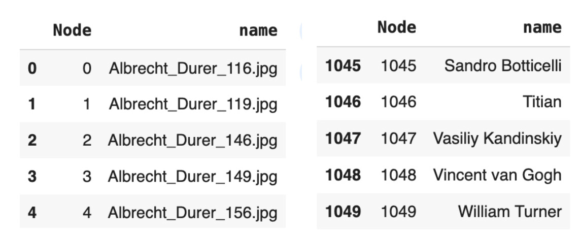 Painting nodes are prepared for the unified Knowledge Graph by mapping each painting to its corresponding artist and assigning unique artist indices.
-
Load painting nodes:The painting graph nodes are loaded from a CSV file, and the column
file_nameis renamed tonamefor consistency. -
Map paintings to artists: A new column,
artist_name, is created by extracting the artist's name from the painting's file name. This assumes the artist's name is the first two words in the file name, separated by underscores. -
Assign unique artist indices: An
artist_indexcolumn is created by dividing the painting node index (Node) by 20 (integer division) and adding an offset of1000. This ensures unique indexing for artists across the graph.
painting_graph_nodes = pd.read_csv("/content/drive/My Drive/Art/painting_graph_nodes.csv")
painting_graph_nodes = painting_graph_nodes.rename(columns={'file_name': 'name'})
painting_artist_graph_nodes=painting_graph_nodes
painting_artist_graph_nodes['artist_name'] = painting_graph_nodes['name']
   .apply(lambda x: x.split('_')[0]+' '+x.split('_')[1] )
painting_artist_graph_nodes['artist_index'] = painting_graph_nodes['Node']
   .apply(lambda x: (x // 20)+1000)
xxx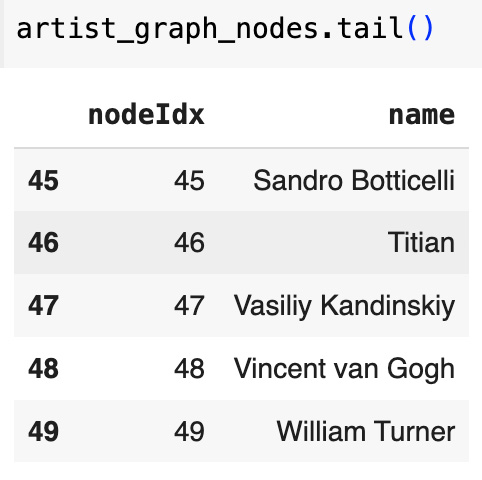
artist_graph_nodes['nodeIdx'] = artist_graph_nodes['nodeIdx'] + 1000
artist_graph_nodes = artist_graph_nodes[['nodeIdx', 'name']]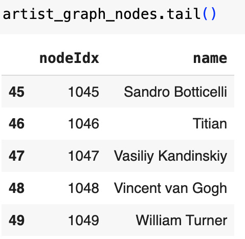
artist_graph_edges['Source'] = artist_graph_edges['Source'] + 1000
artist_graph_edges['Target'] = artist_graph_edges['Target'] + 1000
artist_graph_edges = artist_graph_edges[['Source', 'Target']]painting_artist_graph_nodes=painting_graph_nodes
painting_artist_graph_nodes['artist_name'] =
painting_graph_nodes['name'].apply(lambda x: x.split('_')[0]+' '+x.split('_')[1] )
painting_artist_graph_nodes['artist_index'] =
painting_graph_nodes['Node'].apply(lambda x: (x // 20)+1000)
painting_graph_nodes.tail()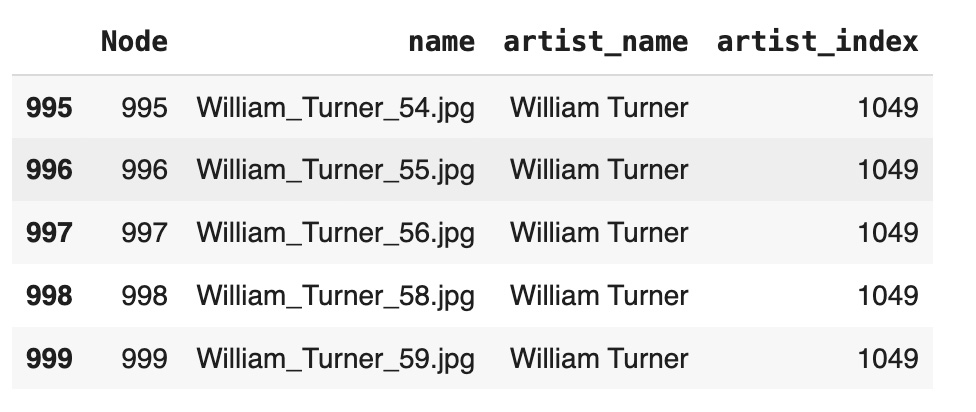
To establish connections between painting nodes and their corresponding artist nodes, edges are created by matching paintings to artists based on their indices:
- Find matching artist nodes: For each painting node, the
artist_indexis used to identify the matching artist node inartist_graph_nodes. - Create edges: For each match, an edge is added between the painting node and the artist node. These edges represent the relationship between a painting and its creator.
- Convert edges to DataFrame: The resulting edges are stored in a DataFrame with
SourceandTargetcolumns, representing the painting and artist nodes, respectively.
The following code implements this process:
edges = []
for _, painting_row in painting_artist_graph_nodes.iterrows():
    artist_matches = artist_graph_nodes[artist_graph_nodes['nodeIdx'] ==
        painting_row['artist_index']]
for _, artist_row in artist_matches.iterrows():
    edges.append((painting_row['Node'], artist_row['nodeIdx']))
painting_artist_graph_edges = pd.DataFrame(edges, columns=['Source', 'Target'])knowledge_graph_nodes = pd.concat([painting_nodes, artist_nodes], ignore_index=True)
knowledge_graph_edges = pd.concat([painting_artist_graph_edges, artist_graph_edges],
ignore_index=True)
knowledge_graph_edges.shape
(1218, 2)Transforming the Unified Graph to DGL Format
The Knowledge Graph is constructed as a DGL graph object. The edges from knowledge_graph_edges are transformed into a PyTorch tensor to define the connections between nodes. These edges are used to create a DGL graph, and self-loops are added to ensure that each node is connected to itself, which can improve GNN performance. The node features are represented by knowledge_graph_embeddings, with each node having a 128-dimensional feature vector. The resulting graph contains 1050 nodes and 2268 edges, making it ready for graph-based learning tasks.unpickEdges=knowledge_graph_edges
edge_index=torch.tensor(unpickEdges[['Source','Target']].T.values)
u,v=edge_index[0],edge_index[1]
gKG=dgl.graph((u,v))
gKG=dgl.add_self_loop(gKG)
gKG.ndata['feat'] = knowledge_graph_embeddings
gKG
Graph(num_nodes=1050, num_edges=2268,
ndata_schemes={'feat': Scheme(shape=(128,), dtype=torch.float32)}
edata_schemes={})GNN Link Prediction Model for Unified Knowledge Graph
The final phase of training involves running the GNN link prediction model for 2000 epochs. During each epoch, the model performs a forward pass to compute node embeddings, calculates scores for positive and negative edges, and computes the loss. Gradients are backpropagated to update model parameters, optimizing the model for link prediction. Progress is logged every 100 epochs, showing the loss to monitor convergence.
After training, the model's performance is evaluated on the test set. Positive and negative edge scores are computed, and the AUC (Area Under the Curve) metric is used to assess the model's ability to distinguish between true and false links. The final AUC score achieved is 0.9007, indicating strong predictive performance.
all_logits = []
for e in range(2000):
    # forward
    h = model(train_g, train_g.ndata['feat'].float())
    pos_score = pred(train_pos_g, h)
    neg_score = pred(train_neg_g, h)
    loss = compute_loss(pos_score, neg_score)
    # backward
    optimizer.zero_grad()
    loss.backward()
    optimizer.step()
    if e % 100 == 0:
        print('In epoch {}, loss: {}'.format(e, loss))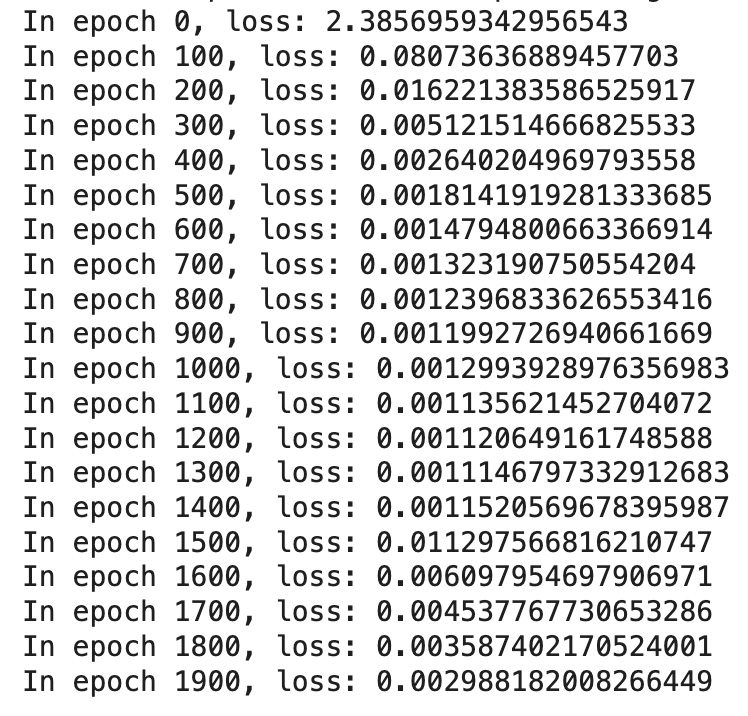
from sklearn.metrics import roc_auc_score
with torch.no_grad():
    pos_score = pred(test_pos_g, h)
    neg_score = pred(test_neg_g, h)
    print('AUC', compute_auc(pos_score, neg_score))
AUC 0.9007130791642577
The node embeddings for the unified Knowledge Graph are saved and reloaded to enable persistent storage and reuse:
- Save embeddings: The node embeddings, represented by the variable
h, are saved to Google Drive as a PyTorch tensor usingtorch.save. This ensures that the embeddings can be preserved for later use. - Load embeddings: The saved embeddings are reloaded from Google Drive using
torch.load. This allows for seamless reuse of the computed embeddings without requiring recomputation.
torch.save(h, '/content/drive/My Drive/Art/artist_knowledge_graph_h.pt')
load_h = torch.load('/content/drive/My Drive/Art/artist_knowledge_graph_h.pt')
Interpreting GNN Link Prediction Model Results
The results of the GNN Link Prediction (LP) model go beyond merely predicting links; they generate embedded vectors for each node in the Unified Knowledge Graph. These vectors, consistent in size, provide high-dimensional representations of the nodes, capturing both contextual and relational information. Such embeddings enable advanced analysis using techniques like cosine similarity, clustering, and building new graph layers, offering deeper insights into the structure and relationships within the graph.
The Unified Knowledge Graph in this study consists of 50 artist nodes and 1000 painting nodes, all encoded as vectors of size 128. The GNN LP model ensures a consistent embedding space across all nodes, enabling seamless analysis and comparisons between different node types.
In this section, we explore two main areas of interpretation:
- Artist-artist relationships: Examining similarities in the embedded vectors to identify shared themes, influences, or overlapping artistic philosophies.
- Painting-painting connections: Analyzing stylistic or contextual similarities between paintings through their embeddings.
Model Results Analysis
In this step, we calculate the cosine similarity between all pairs of nodes in the Unified Knowledge Graph using their embedded vectors. The similarity scores, generated by a PyTorch function, quantify the relationships between nodes based on their high-dimensional embeddings. The result is stored in a DataFrame containing 1,102,500 rows, representing all possible pairs of 1,050 nodes (50 artists and 1,000 paintings). Each row includes the indices of the two nodes and their corresponding similarity score, which serves as the foundation for analyzing relationships between nodes in the graph.cosine_scores_gnn = pytorch_cos_sim(load_h, load_h)
pairs_scores = []
for i in range( len(cosine_scores_gnn)):
for j in range(len(cosine_scores_gnn)):
pairs_scores.append({
'idx1': i,
'idx2': j,
'score': cosine_scores_gnn[i][j].item() # Use `.item()` for scalar tensors
})
df=pd.DataFrame(pairs_scores)
df.shape
(1102500, 3)This step enhances the similarity DataFrame by joining node information from the Unified Knowledge Graph. For each pair of indices (idx1 and idx2), node metadata such as names and types are added, providing contextual information about the nodes involved in each similarity computation.
Key steps include:
- Joining node information: The
idx1andidx2columns are matched with thenodeIdxcolumn in the Knowledge Graph nodes DataFrame, adding relevant details about each node. - Renaming columns: After the join, node metadata (
nodeNameandnodeType) is renamed tonode1_name,node1_type,node2_name, andnode2_typefor clarity. - Dropping redundant columns: Extra columns from the join (
nodeIdx_xandnodeIdx_y) are removed, keeping the DataFrame clean and focused on relevant information.
The resulting DataFrame includes enriched details about each pair of nodes, laying the groundwork for deeper analysis of relationships within the graph.
df = df.merge(knowledge_graph_nodes, left_on='idx1', right_on='nodeIdx', how='left')
df = df.rename(columns={'nodeName': 'node1_name', 'nodeType': 'node1_type'})
df = df.merge(knowledge_graph_nodes, left_on='idx2', right_on='nodeIdx', how='left')
df = df.rename(columns={'nodeName': 'node2_name', 'nodeType': 'node2_type'})
df = df.drop(columns=['nodeIdx_x', 'nodeIdx_y'])
graph_pairs = df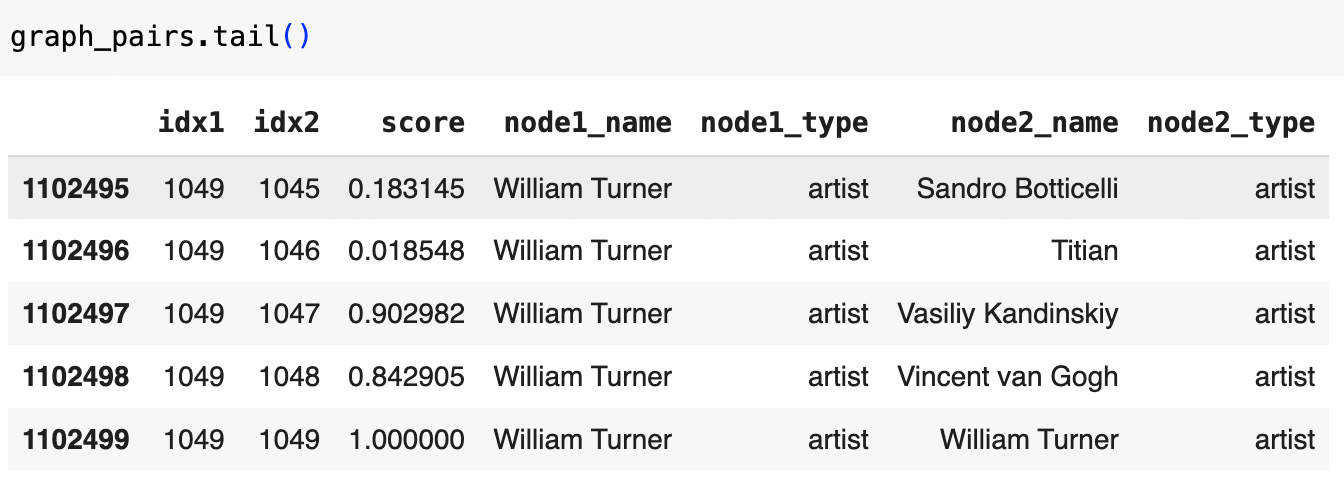
Cosine Similarity Score Distributions
The GNN Link Prediction model generates similarity scores for each pair of nodes in the Unified Knowledge Graph. These scores represent the relationships between nodes and provide insights into the structure and connections within the graph.
For all node pairs, excluding self-loops, scores range from -0.515 to 1.000, with a mean of approximately 0.460. This indicates that many pairs exhibit moderate similarity, while higher scores highlight stronger relationships.
filtered_graph_pairs = graph_pairs[graph_pairs['idx1'] != graph_pairs['idx2']]
overall_scores = filtered_graph_pairs['score']
overall_stats = overall_scores.describe()
print("Overall Score Distribution:\n", overall_stats)
Overall Score Distribution:
count 1101450.000000
mean 0.460064
std 0.337415
min -0.515314
25% 0.217390
50% 0.471504
75% 0.744774
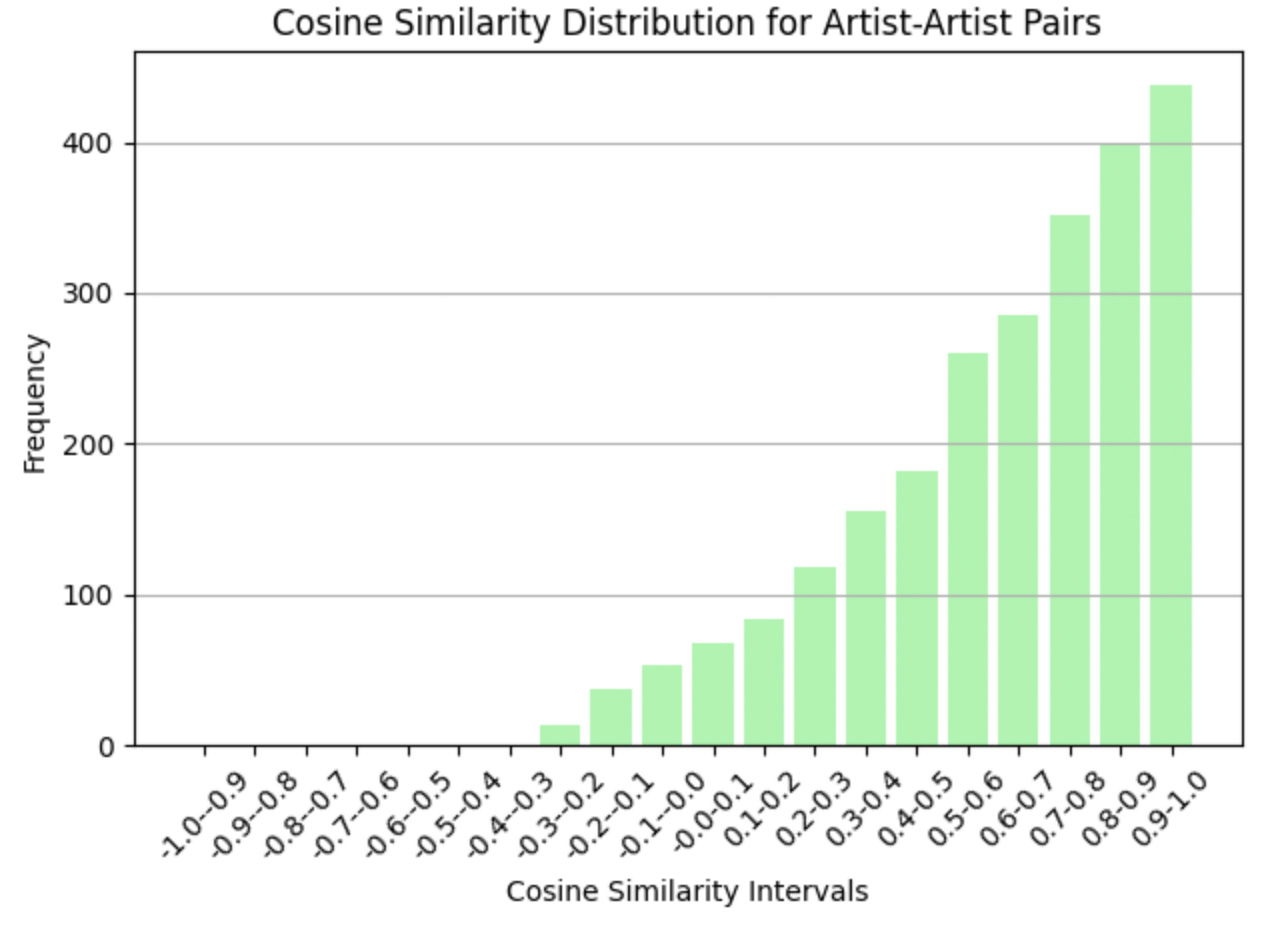
max 1.000000Artist-artist pairs show a higher mean score of 0.621, reflecting strong semantic relationships such as shared influences or overlapping styles.
artist_artist_pairs = filtered_graph_pairs[
    (filtered_graph_pairs['node1_type'] == 'artist') & (filtered_graph_pairs['node2_type'] == 'artist')
]
artist_artist_scores = artist_artist_pairs['score']
artist_stats = artist_artist_scores.describe()
print("Artist-Artist Score Distribution:\n", artist_stats)
Artist-Artist Score Distribution:
 count    2450.000000
mean        0.621267
std         0.291015
min        -0.281765
25%         0.455145
50%         0.688079
75%         0.860471
max 0.992316painting_painting_pairs = filtered_graph_pairs[
(filtered_graph_pairs['node1_type'] == 'painting') & (filtered_graph_pairs['node2_type'] == 'painting')
]
painting_scores = painting_painting_pairs['score']
painting_stats = painting_scores.describe()
print("Painting-Painting Score Distribution:\n", painting_stats)
Painting-Painting Score Distribution:
count 999000.000000
mean 0.477173
std 0.338798
min -0.515314
25% 0.232907
50% 0.492818
75% 0.769807
max 1.000000These distributions reveal the model's ability to capture meaningful relationships across different types of nodes, setting the stage for deeper analysis of highly connected and less connected nodes. Such insights are valuable for exploring relationships in art and uncovering hidden patterns.
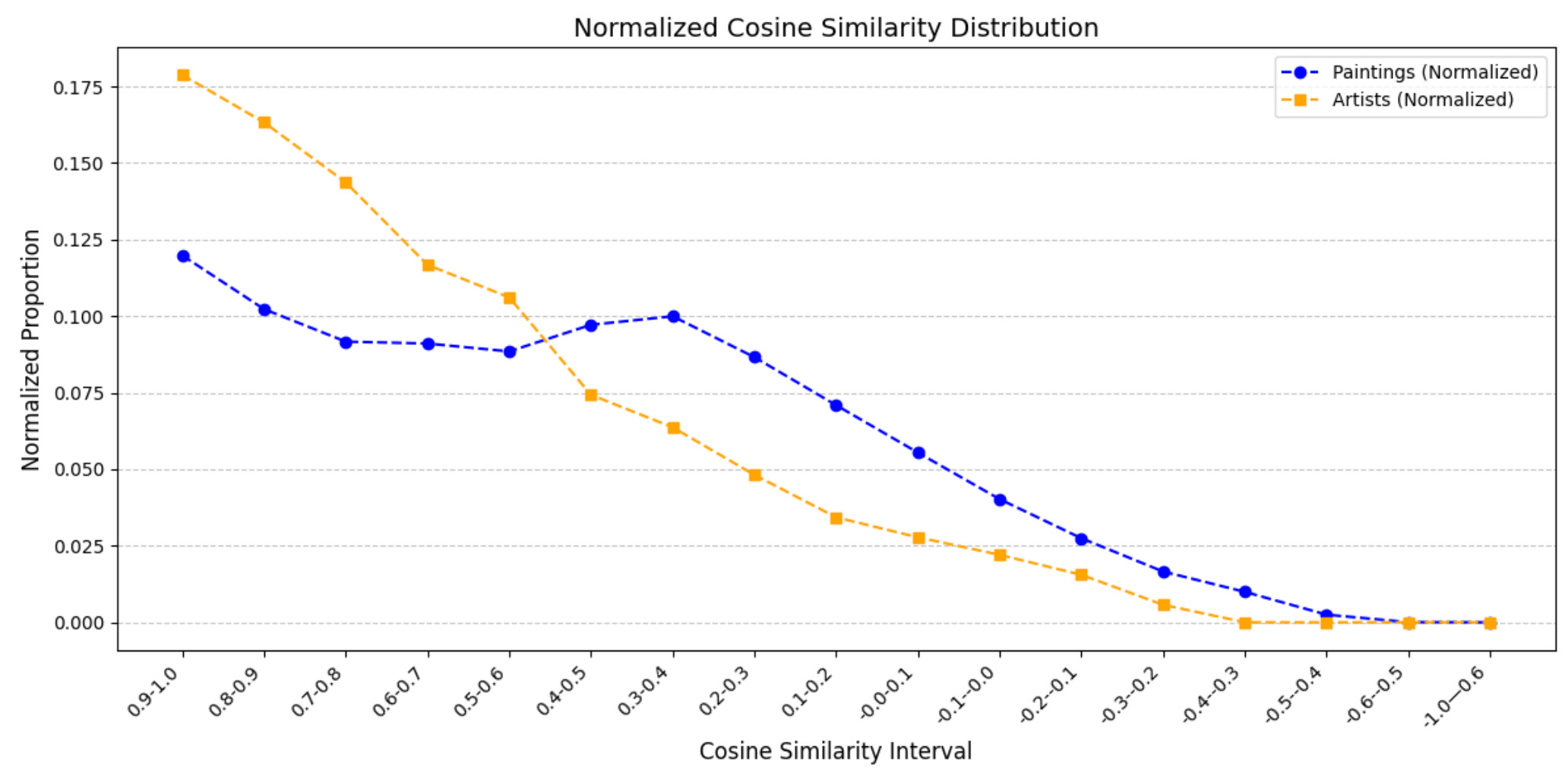
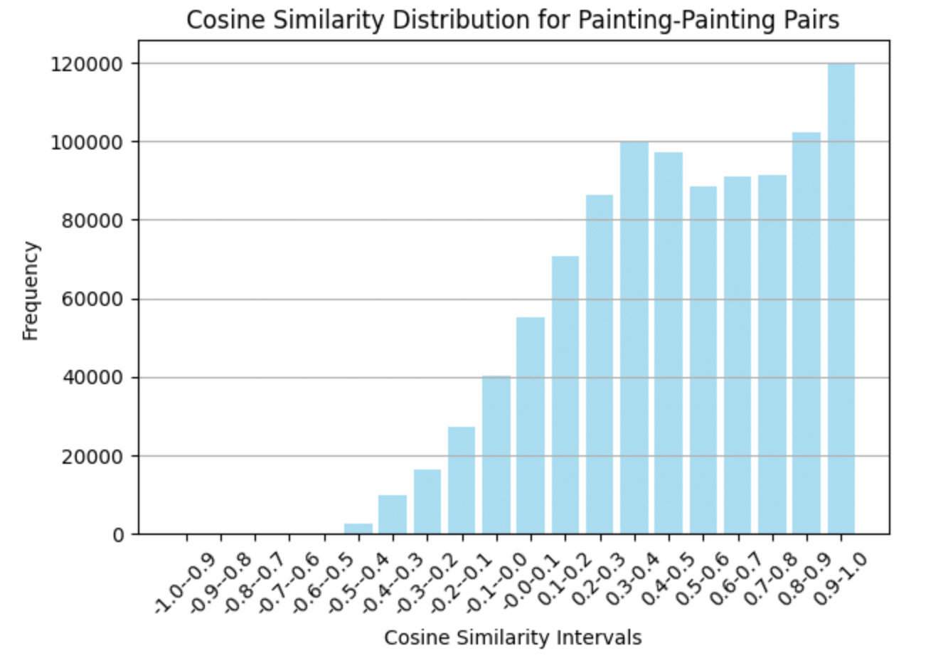
This analysis explores the distribution of cosine similarity scores for painting-painting pairs. The scores are grouped into intervals ranging from -1.0 to 1.0 in steps of 0.1. Data is filtered to include only painting-painting connections, and a histogram visualizes the frequency of pairs within each interval. The results highlight a concentration of pairs in higher intervals (e.g., 0.9-1.0), suggesting strong stylistic or thematic similarities between many paintings. In contrast, lower intervals reveal fewer connections, emphasizing weaker or negative correlations.
import numpy as np
import pandas as pd
import matplotlib.pyplot as plt
bins = np.arange(-1.0, 1.1, 0.1)
bins[-1] = bins[-1] + 0.001
painting_painting_pairs = filtered_graph_pairs[
    (filtered_graph_pairs['node1_type'] == 'painting') &
    (filtered_graph_pairs['node2_type'] == 'painting')
]
frequency, bin_edges = np.histogram(painting_painting_pairs['score'], bins=bins)
intervals = [f"{round(bin_edges[i], 1)}-{round(bin_edges[i + 1], 1)}" for i in range(len(bin_edges) - 1)]
freq_df = pd.DataFrame({'Interval': intervals, 'Frequency': frequency})
freq_df = freq_df.iloc[::-1]
print(freq_df)
plt.bar(freq_df['Interval'], freq_df['Frequency'], color='skyblue', alpha=0.7)
plt.xticks(rotation=45)
plt.title("Cosine Similarity Distribution for Painting-Painting Pairs")
plt.xlabel("Cosine Similarity Intervals")
plt.ylabel("Frequency")
plt.gca().invert_xaxis()  # Invert x-axis for descending order
plt.grid(axis='y')
plt.tight_layout()
plt.show()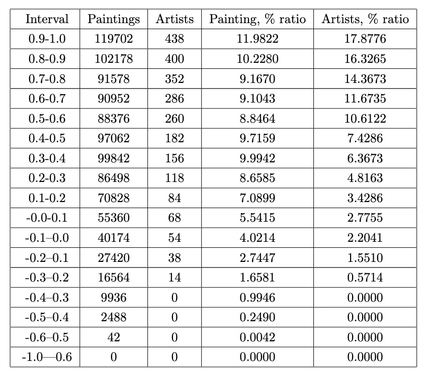
Painting-Painting Connections
This section focuses on analyzing connections between paintings based on their similarity scores, emphasizing relationships that span across different artists. By filtering and enriching the DataFrame, we can better understand how paintings from various artists relate to one another.
Key steps include:
- Filtering painting-painting pairs: Rows where both nodes are of type
paintingare extracted, creating a subset of the data that exclusively examines relationships between paintings. - Extracting artist names: For each painting, the artist’s name is derived from the file name by splitting the string and capturing the relevant segment. The artist names are stored in new columns
artist1andartist2. - Cross-artist connections: Connections between paintings created by different artists are identified by filtering for pairs where
artist1is not equal toartist2. Additionally, only unique pairs are retained by ensuringidx1 < idx2.
painting_pairs=df[(df['node1_type']=='painting') & (df['node2_type']=='painting')]
painting_pairs['artist1']=painting_pairs['node1_name'].apply(lambda x: x.split('_')[-2])
painting_pairs['artist2']=painting_pairs['node2_name'].apply(lambda x: x.split('_')[-2])
dfp=painting_pairs
Cross-Artist Painting Connections Analysis
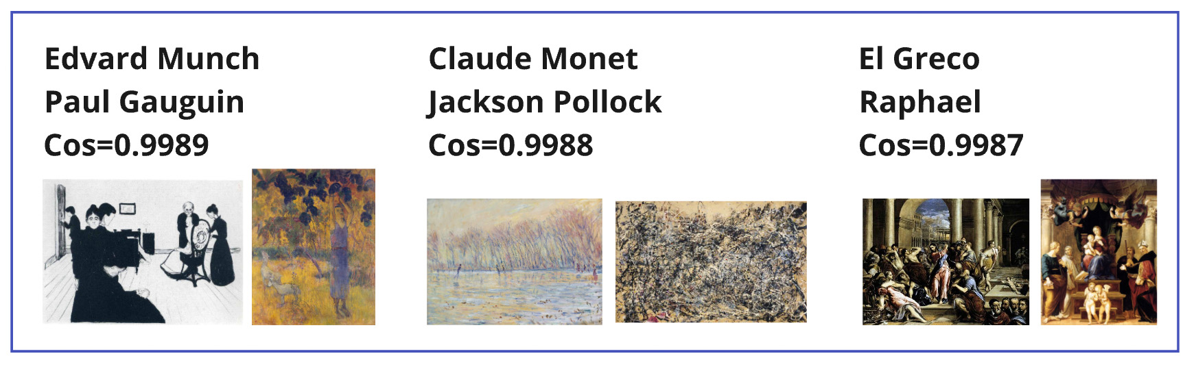
The analysis focuses on identifying connections between paintings created by different artists, highlighting stylistic or thematic similarities. By filtering pairs of paintings where the creators are distinct, and ensuring unique combinations, we analyzed a total of 490,000 cross-artist connections. The top-scoring pairs based on cosine similarity are presented below, offering insights into overlapping influences and shared artistic elements.
diffArtistPaintings= dfp[(dfp['artist1']!=dfp['artist2']) & (dfp['idx1'] < dfp['idx2'])]
diffArtistPaintings.shape : (490000, 9)
diffArtistPaintings.sort_values(by='score').tail(9)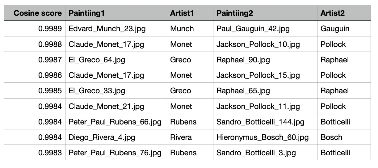 Observations:
- Stylistic Overlaps: High similarity scores suggest shared stylistic elements or thematic connections between paintings, even from different movements.
- Artistic Influence: These links may indicate underlying inspirations or techniques shared across eras or artistic philosophies.
- Applications: The insights can support art recommendations, historical analyses, or new narratives in understanding artistic relationships.
Exploring Painting-Painting Connections Within the Same Artist
This table highlights painting-painting connections within the works of the same artist, showcasing the least similar pairs based on cosine similarity scores derived from the GNN embeddings.
artistPaintings= dfp[(dfp['artist1']==dfp['artist2']) & (dfp['idx1'] < dfp['idx2'])]
artistPaintings.sort_values(by='score').head(11)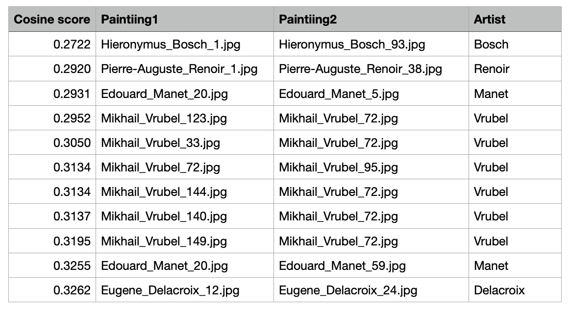 Key Observations
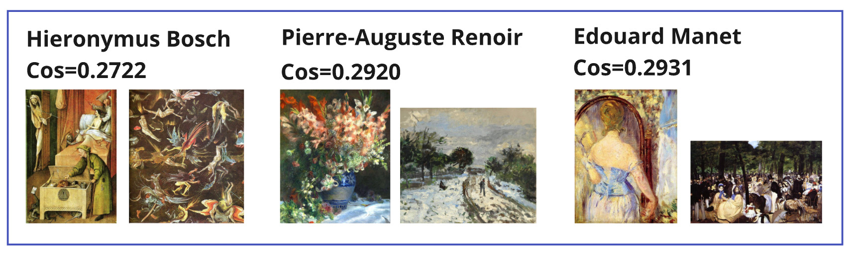
- Low Cosine Similarity Within Same Artist's Works:
- Hieronymus Bosch has the lowest similarity score (0.2722), indicating significant variation between the chosen paintings, likely due to differences in themes or styles.
- Pierre-Auguste Renoir and Edouard Manet also have scores near 0.29, reflecting diversity in artistic elements.
- Mikhail Vrubel Dominates: The table features multiple pairs from Mikhail Vrubel, with scores ranging from 0.2952 to 0.3195, highlighting his stylistic versatility.
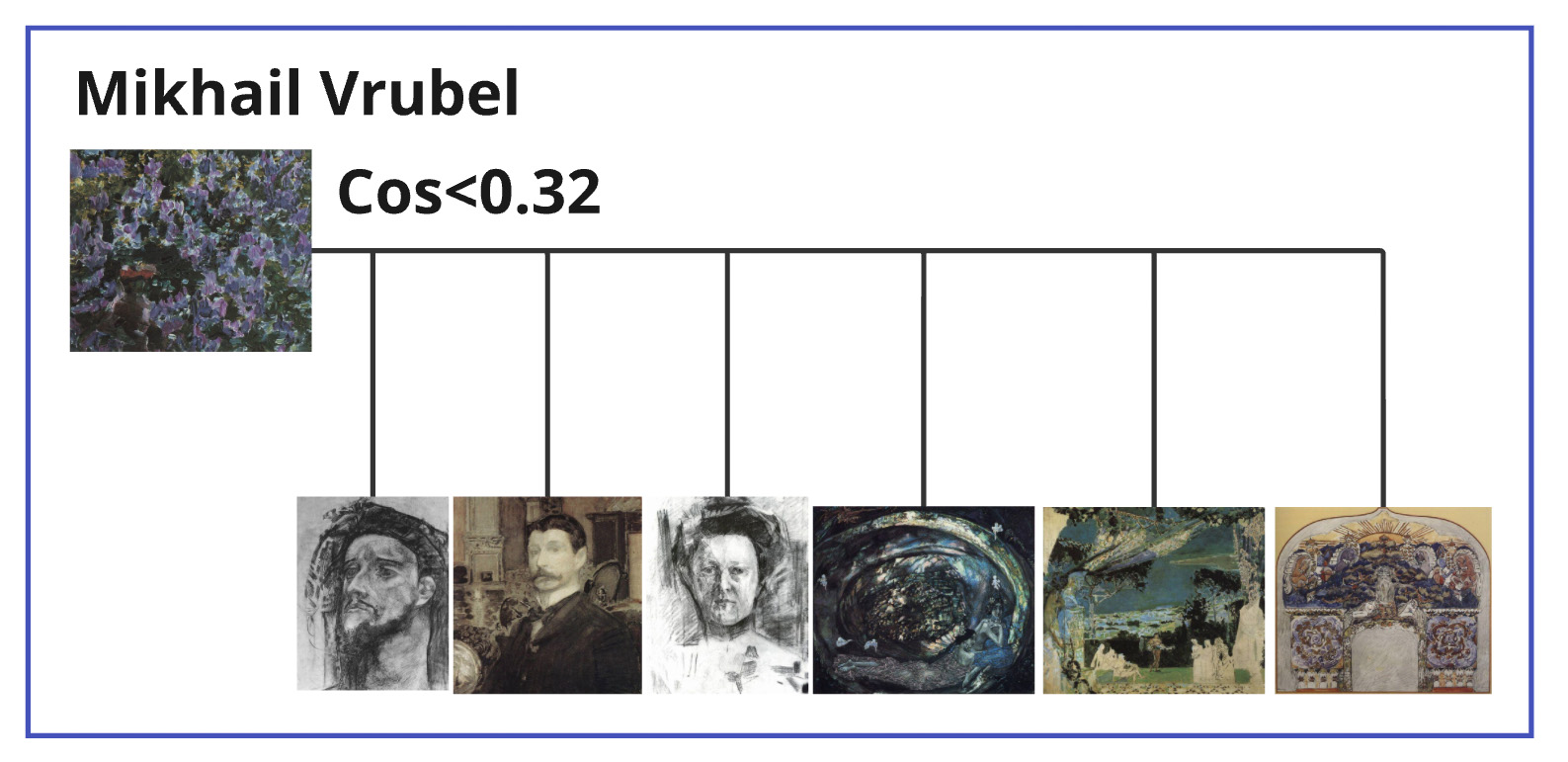 This visualization highlights the painting "Lilac" by Mikhail Vrubel, which exhibits a low cosine similarity (<0.32) to his other works. This deviation offers insight into how specific pieces can stand apart from an artist's typical style, enriching our understanding of their creative range and versatility.
The low similarity scores between paintings of the same artist emphasize stylistic versatility or exploration within their body of work. These results provide valuable insights into the evolution and experimentation of individual artists, offering a deeper understanding of their creative journeys.
Artist-Artist Connections
This analysis explores the relationships between artists by categorizing their connections based on cosine similarity scores and metadata such as shared genres or nationalities. First, pairs of artist nodes were isolated and merged with existing edge data to identify relationships such as shared genres or nationalities. Missing values in thegenre and nationality columns were replaced with "None" to standardize the dataset for further processing.
artist_pairs=df[(df['node1_type']=='artist') & (df['node2_type']=='artist')]
combined_df['genre'] = combined_df['genre'].fillna('None')
combined_df['nationality'] = combined_df['nationality'].fillna('None')
combined_df = pd.merge(
    artist_pairs,
    artist_edges,
    on=['idx1', 'idx2'],
    how='left'
)
To better understand the nature of artist connections, a new column, edge_type, was introduced to classify relationships into the following categories:
- Genre: When artists share a common artistic style or movement.
- Nationality: When artists belong to the same country.
- Both: When artists share both genre and nationality.
- None: When no direct connection exists in the provided metadata.
This categorization offers valuable insights into the nature of artist-artist relationships, helping uncover patterns and anomalies within the graph.
def determine_edge_type(row):
    if row['genre'] != 'None' and row['nationality'] != 'None':
        return 'both'
    elif row['genre'] != 'None':
        return 'genre'
    elif row['nationality'] != 'None':
        return 'nationality'
    else:
        return 'none'
combined_df['edge_type'] = combined_df.apply(determine_edge_type, axis=1)
combined_df[combined_df['edge_type']!='none'].tail(11)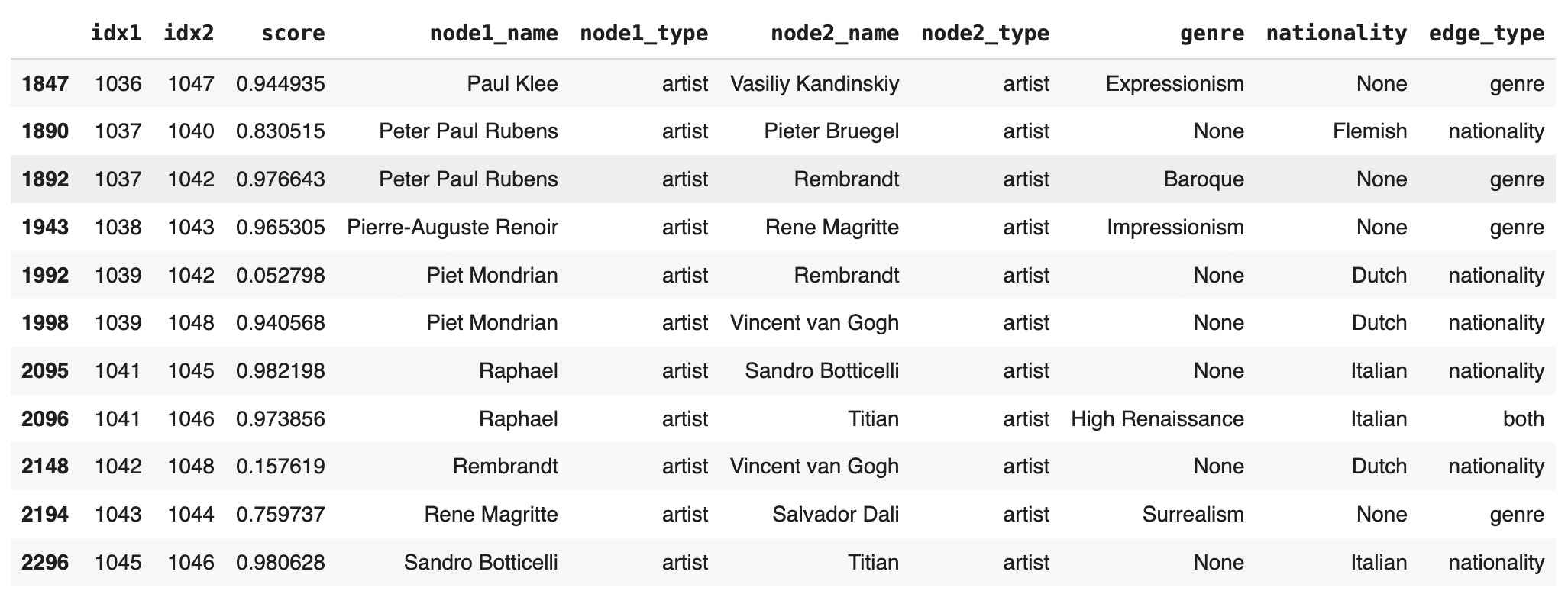
stats = combined_df.groupby('edge_type')['score']
  .agg(['mean', 'median', 'min', 'max', 'std']).reset_index()
print("Statistics by Edge Type:")
print(stats)
Statistics by Edge Type:
     edge_type      mean    median       min       max       std
0         both  0.751972  0.790473  0.345487  0.989279  0.210772
1        genre  0.817520  0.864702  0.260232  0.978745  0.149252
2  nationality  0.719641  0.791969  0.052798  0.992316  0.245162
3 none 0.617343 0.685730 -0.281765 1.000000 0.296322plt.figure(figsize=(8, 5))
order = ['both', 'genre', 'nationality', 'none'] # Specify the desired order
sns.boxplot(x='edge_type', y='score', data=combined_df, order=order, color='lightgray') # Use single color
plt.title("Score Distribution by Edge Type", fontsize=14)
plt.xlabel("Edge Type", fontsize=12)
plt.ylabel("Score", fontsize=12)
plt.show()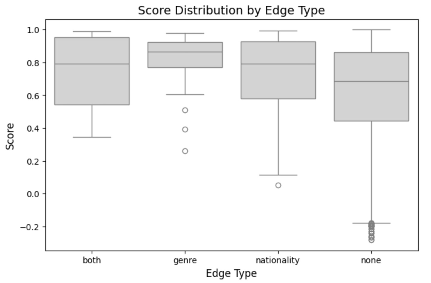
In this analysis, we focus on understanding the relationships between artist nodes by exploring similarity scores for different edge types. By examining both high and low scores, we gain insights into hidden connections and variations among artists.
Low Scores with 'Both'
Even when artists share both genre and nationality, low similarity scores reveal nuanced differences. These pairs demonstrate the diversity that can exist even within closely related artistic and cultural contexts.
df=combined_df
low_scores_both = df[(df['edge_type'] == 'both') & (df['idx2'] > df['idx1'])]
print("Low scores with 'genre' edge type:")
low_scores_both.sort_values(by='score').head(7)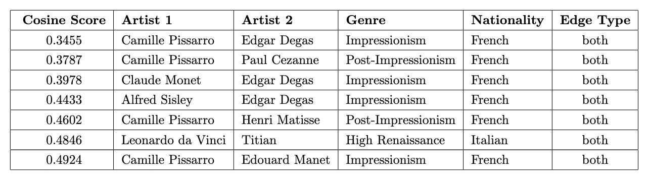 With the exception of Titian and Leonardo da Vinci, all pairs are French artists from Impressionism or Post-Impressionism, yet their low cosine similarity scores highlight nuanced stylistic differences within these closely related movements.
Low Scores with 'Nationality'
Artists sharing the same nationality but exhibiting weak similarities highlight diversity within a shared cultural framework. These cases may represent unique interpretations or individualistic approaches despite shared backgrounds.
low_scores_nationality = df[(df['edge_type'] == 'nationality') & (df['idx2'] > df['idx1'])]
print("Low scores with 'nationality' edge type:")
low_scores_nationality.sort_values(by='score').head(11)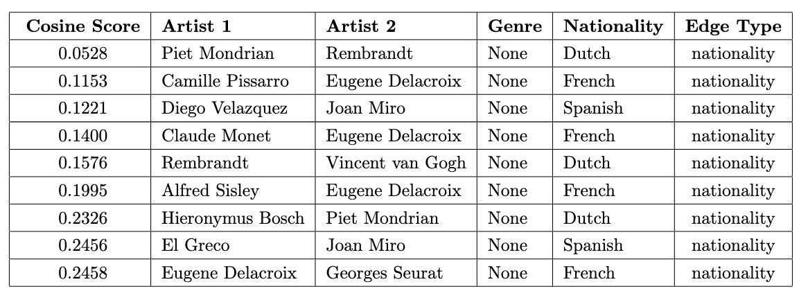 The low cosine similarity scores between artists of the same nationality often reflect differences in time periods and artistic movements. For example, Rembrandt and Piet Mondrian represent vastly different eras—17th-century Baroque and 20th-century Abstract art—while Camille Pissarro and Eugene Delacroix belong to distinct movements like Impressionism and Romanticism. These temporal and stylistic disparities highlight the diversity within shared cultural backgrounds.
Low Scores with 'Genre'
For artist pairs connected by the same genre but showing low similarity scores, we explore how artists within a single genre can differ significantly in their styles, techniques, or approaches to art.
low_scores_genre = df[(df['edge_type'] == 'genre') & (df['idx2'] > df['idx1'])]
print("Low scores with 'genre' edge type:")
low_scores_genre.sort_values(by='score').head()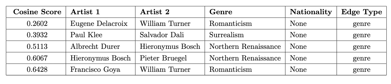 For artists connected by the same genre, even the lowest cosine similarity scores are relatively high, indicating a baseline level of shared characteristics. However, these pairs still highlight stylistic diversity within the same genre, such as the contrasting approaches of Eugene Delacroix and William Turner in Romanticism or the differences between Albrecht Dürer and Hieronymus Bosch in the Northern Renaissance.
High Scores with 'None'
Artists with no shared genre or nationality but high similarity scores reveal unexpected connections. These relationships may indicate shared influences, overlapping themes, or stylistic similarities that are not captured by explicit attributes.
high_scores_none = df[(df['edge_type'] == 'none') & (df['idx2'] > df['idx1'])]
print("High scores with 'none' edge type:")
high_scores_none.sort_values(by='score',ascending=False).head(7)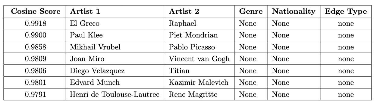 These high scores, despite no overlaps in genre or nationality, suggest deeper, unrecognized influences or thematic and stylistic parallels that transcend traditional classifications, warranting further exploration. One such connection is between Pablo Picasso (1881–1973), the Spanish pioneer of Cubism, and Mikhail Vrubel (1856–1910), a Russian Symbolist painter. Although they lived in different periods and represented contrasting artistic movements, a historical link bridges their work. In 1906, Sergey Diaghilev brought Vrubel’s works to Paris, where they captured the admiration of a young Pablo Picasso.
Conclusion
This study presented a Unified Knowledge Graph framework that combines text and image data to explore artistic relationships. By utilizing Graph Neural Networks (GNNs) for embedding and link prediction, we uncovered meaningful connections within and across artist and painting nodes, revealing both expected patterns and surprising insights.
Key findings include:
- Cross-Artist Painting Connections: Identified thematic overlaps and stylistic diversity between works created by different artists.
- Artist-Specific Variations: Highlighted the evolution and experimentation within individual artists' portfolios, showcasing their creative range.
- Unexpected Influences: Discovered surprising connections, such as historical links between Pablo Picasso and Mikhail Vrubel, demonstrating the broader potential of this approach.
The Unified Knowledge Graph provides a powerful tool for analyzing complex datasets, offering fresh perspectives on art history. It also paves the way for applications in recommendation systems, classification tasks, and cultural analysis. Future work will focus on expanding the graph with additional data types and improving model interpretability.