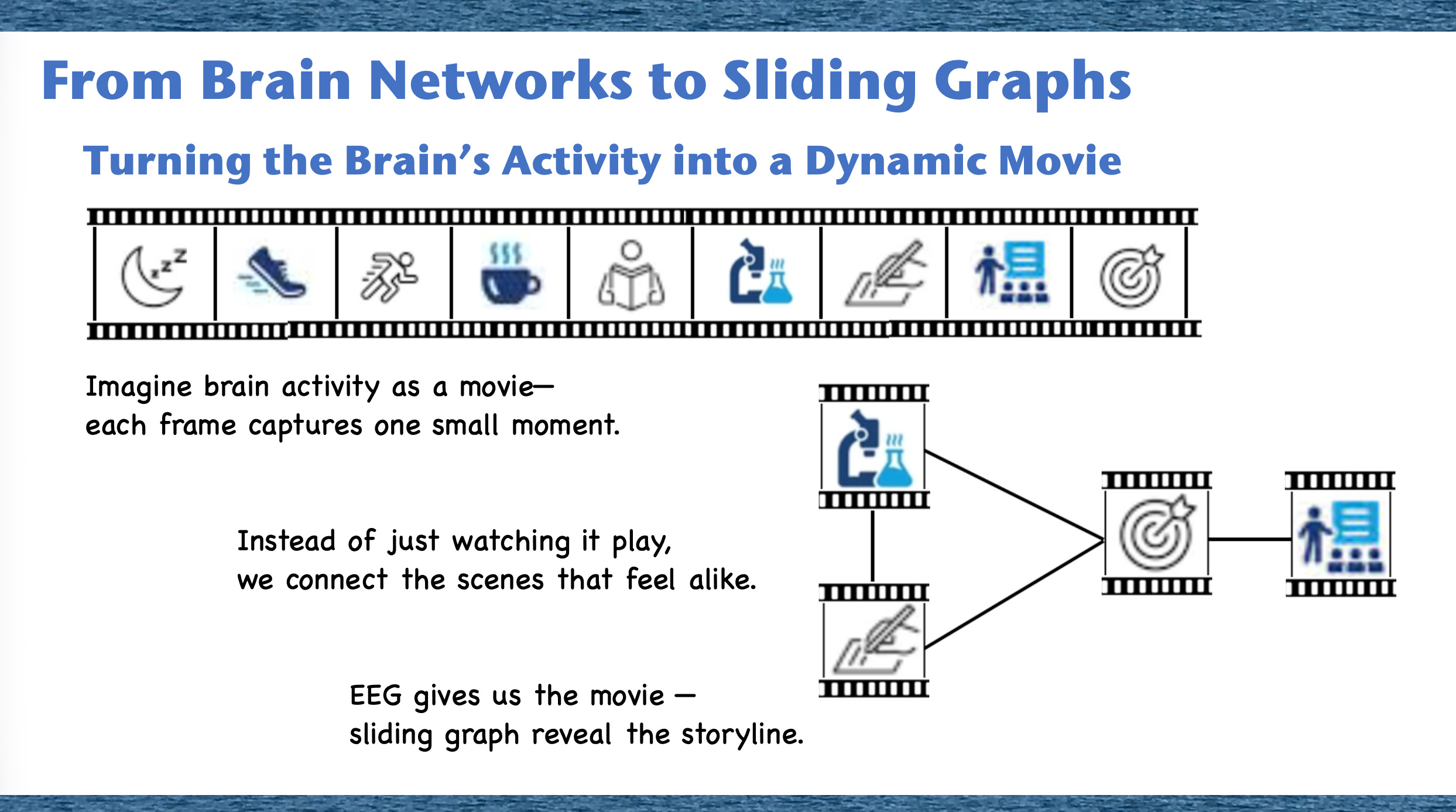
Sliding Graphs: Watching Signals Change Like a Movie
Sliding graphs are a way to let AI watch how a signal behaves over time, not just look at a summary. Instead of treating a long recording as one big block, we break it into many small, overlapping moments and let AI see which moments look alike and which don’t. Put together, these moments form an evolving map of the signal, showing when things are calm, when they shift, and when something unusual starts to happen. We illustrate this with EEG sleep vs rest, but the same idea works for machines, sensors, markets, climate, or any long signal—anywhere you want AI to say not only what is happening, but when things start to change.
Conference
The work “Time Aligned Sliding Graph Embeddings for Dynamic Time Series Analysis” was presented at Brain Informatics 2025 in Bari, Italy, on 11 November 2025. The corresponding paper is not yet published in archival proceedings.
Exploring EEG Through Graph-Based Methods
Over the years, we are looking to uncover the secrets of brain connectivity using EEG data. Our work has evolved from traditional graph analysis techniques to cutting-edge Graph Neural Networks (GNNs), each step uncovering deeper insights into neural dynamics. Let’s take a closer look at these studies.
Study 1: Traditional Graph Analysis
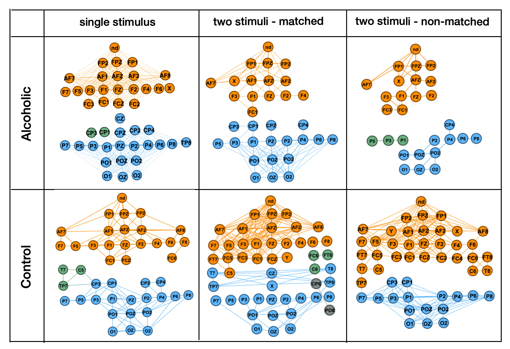
Our journey began with a traditional graph analysis approach. In this study, we constructed connectivity graphs from EEG trials using cosine similarity between channels. Each graph’s nodes represented EEG electrodes, and the edges reflected their functional connectivity.
Key Findings:
- Differences in connectivity patterns emerged between the Alcoholic and Control groups, providing insights into altered neural activity.
- Graph features like clustering coefficients and edge density helped highlight these differences.
- However, traditional methods struggled to distinguish subtle variations, particularly in single-stimulus conditions, prompting the need for more advanced techniques.
For a deeper dive into this work, check out our post “EEG Patterns by Deep Learning and Graph Mining” or refer to the paper Time Series Pattern Discovery by Deep Learning and Graph Mining.
Study 2: Graph Neural Networks for Trial Classification
On the second study, we introduced Graph Neural Networks (GNNs) to analyze EEG data at the trial level. Each graph represented an entire EEG trial, encapsulating the connectivity across all channels.
Why GNNs? GNNs brought a new level of sophistication by enabling the model to learn spatial relationships and connectivity dynamics within the graph.
Key Findings:
- Improved Classification Accuracy: GNN Graph Classification models significantly outperformed traditional methods in differentiating between Alcoholic and Control groups.
- Enhanced Connectivity Insights: Subtle variations in connectivity, previously missed, were captured.
- Challenges: Misclassifications within the Control group highlighted the complexity of EEG connectivity patterns.
This approach is detailed further in our post “GNN Graph Classification for EEG Pattern Analysis” or refer to the paper Enhancing Time Series Analysis with GNN Graph Classification Models.
Study 3: Graph Neural Networks for Link Prediction
In our third study, the focus shifted to link prediction, using GNNs to analyze node- and edge-level connectivity. A unified graph constructed from EEG electrode distances was used to predict connectivity dynamics.
Key Findings:
- Revealing Hidden Connectivity: GNN Link Prediction models highlighted relationships between electrodes that were previously unobserved.
- Node Importance: Certain electrodes emerged as more central to connectivity patterns.
- Limitations: This method focused primarily on short-term EEG segments, leaving the dynamics of long-term recordings unexplored.
For more on this work, check out our “Graph Neural Networks for EEG Connectivity Analysis” or refer to the paper Graph Neural Networks in Action: Uncovering Patterns in EEG Time Series Data. 1st International Workshop on Artificial Intelligence for Neuroscience (IWAIN’24), pp. 4–15.
Looking Ahead: Current Study
This study applies GNN Sliding Graph Classification to long-time EEG series, capturing evolving neural activity during sleep and rest. This approach reveals extended brain states, uncovering transitions and sustained neural processes, offering deeper insights into EEG dynamics over time.
Imagine moving a sliding window through EEG data—like watching a movie, scene by scene. Each window captures a brief moment in time. Now imagine building a graph that doesn’t just follow the timeline, but connects moments that belong to the same theme—even if they’re far apart. Like linking “research” and “presentation” as part of the same goal. That graph becomes a story—showing how different moments are connected by meaning, not just time.
GNN Sliding Graph Classification: Introduction
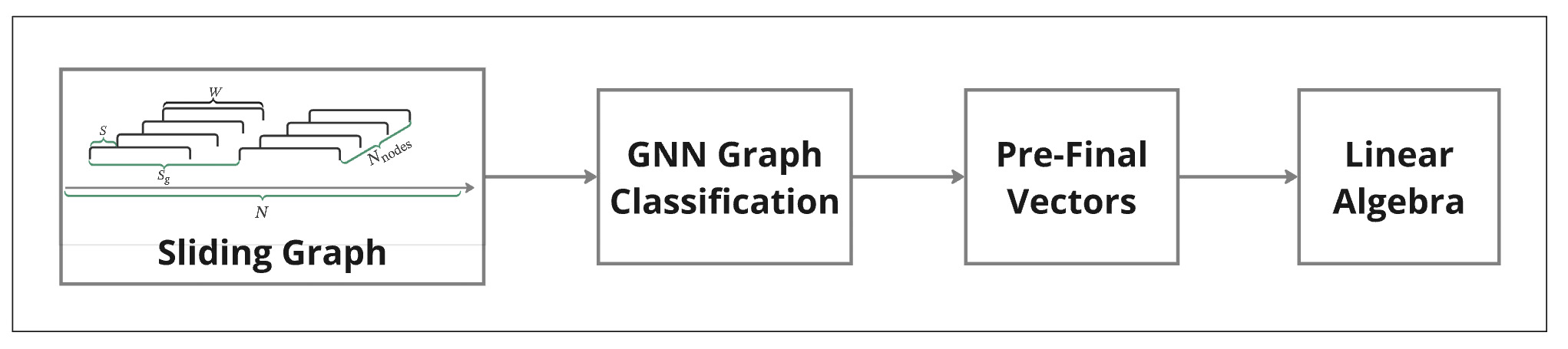
In our previous work, we introduced two key methods for time series analysis. The methodology consists of three key steps:
- Sliding Graph Construction: Transform time series data into graph structures by segmenting it into overlapping windows. Each graph captures localized temporal and spatial relationships, representing distinct patterns over the chosen time frame.
- GNN Graph Classification: Utilize GNNs to classify these graphs, extracting high-level features from their topology while preserving the structural and temporal dependencies in the data.
- Pre-final Vectors: Obtain graph embeddings (pre-final vectors) from the GNN Graph Classification model during classification. These embeddings represent the learned topological features and are further analyzed to reveal temporal and structural patterns in the time series.
Both methods were successfully applied to climate time series data, revealing complex patterns in large-scale datasets. However, these techniques have never been combined in a single study.
In this study, we integrate these approaches and apply them to EEG time series data, specifically in the context of sleep studies. EEG analysis presents unique challenges, requiring methods that can detect both long-term trends and local brain connectivity changes. By leveraging sliding graph construction and pre-final vector extraction, we aim to uncover hidden EEG patterns that traditional signal processing techniques might miss.
Objectives of This Study
- Demonstrate the effectiveness of graph-based models for long-duration biomedical signal analysis.
- Validate the generalizability of GNN Sliding Graph Classification and Pre-Final Vectors beyond climate data, applying them to neuroscience.
This approach bridges sliding window techniques and graph-based modeling, providing a powerful framework for analyzing complex temporal EEG data. By capturing both localized and global topological patterns, it enhances our understanding of brain activity dynamics during sleep.
For more detailed information about GNN Sliding Graphs, look at our post “Sliding Window Graph in GNN Graph Classification” or refer to the paper GNN Graph Classification for Time Series: A New Perspective on Climate Change Analysis.
For information about catching embedded graphs, look at our post “Unlocking the Power of Pre-Final Vectors in GNN Graph Classification” or refer to the paper Utilizing Pre-Final Vectors from GNN Graph Classification for Enhanced Climate Analysis.
Methods
Pipeline
Our pipeline for Graph Neural Network (GNN) Graph Classification consists of several stages.
- The process begins with data input, where EEG data representing brain activity during sleep and rest states is collected.
- Graph construction:
- Sliding window method: Segments time series data into overlapping graphs to maintain temporal structure.
- Virtual nodes: Act as central hubs, improving model accuracy and information flow.
- The GNN model classifies these graphs based on detected patterns.
- To enhance interpretability, pre-final vectors are extracted from the model, capturing deeper structural information before classification.
- Linear algebra analysis applies cosine similarity computations to these embeddings, uncovering connectivity trends over time.
- This approach enables effective modeling of long-duration EEG dynamics by integrating graph-based learning with temporal analysis techniques.
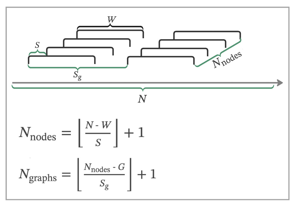
Sliding Graph Construction
In our previous study, GNN Graph Classification for Time Series: A New Perspective on Climate Change Analysis, we introduced an approach to constructing graphs using the Sliding Window Method.
Sliding Window Method
- Nodes: Represent data points within each sliding window, with features reflecting their respective values.
- Edges: Connect pairs of points to preserve the temporal sequence and structure.
- Labels: Assigned to detect and analyze patterns within the time series.
Methodology for Sliding Window Graph Construction
Data to Graph Transformation
Time series data is segmented into overlapping windows using the sliding window technique. Each segment forms a unique graph, allowing for the analysis of local temporal dynamics.
In these graphs:
- Nodes: Represent data points within the window, with features derived from their values.
- Edges: Connect pairs of nodes to maintain temporal relationships.
Key Parameters:
- Window Size (W): Determines the size of each segment.
- Shift Size (S): Defines the degree of overlap between windows.
- Edge Definitions: Tailored to the specific characteristics of the time series, helping detect meaningful patterns.
Node Calculation
For a dataset with N data points, we apply a sliding window of size W with a shift of S to create nodes. The number of nodes, Nnodes, is calculated as:
Graph Calculation
With the nodes determined, we construct graphs, each comprising G nodes, with a shift of Sg between successive graphs. The number of graphs, Ngraphs, is calculated by:
Graph Construction
Cosine similarity matrices are generated from the time series data and transformed into graph adjacency matrices.
- Edge Creation: Edges are established for vector pairs with cosine values above a defined threshold.
- Virtual Nodes: Added to ensure network connectivity, enhancing graph representation.
This framework effectively captures both local and global patterns within the time series, yielding valuable insights into temporal dynamics.
Graph Classification
We employ the GCNConv model from the PyTorch Geometric Library for GNN Graph Classification tasks. This model performs convolutional operations, leveraging edges, node attributes, and graph labels to extract features and analyze graph structures comprehensively.
By combining the sliding window technique with Graph Neural Networks, our approach offers a robust framework for analyzing time series data. It captures intricate temporal dynamics and provides actionable insights into both local and global patterns, making it particularly well-suited for applications such as EEG data analysis. This method allows us to analyze time series data effectively by capturing both local and global patterns, providing valuable insights into temporal dynamics.
Pairwise GNN Sliding Graph Classification
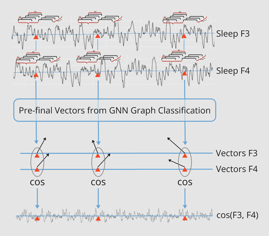
This figure illustrates the process of pairwise GNN Sliding Graph Classification, where pairs of long time series are analyzed using graph-based methods to capture dynamic connectivity patterns. Channels F3-F4 during sleep are used as an illustrative example. Below is a breakdown of the methodology:
- Input Time Series as Pairs: Two long time series (e.g., Sleep F3 and Sleep F4) are taken as input, each representing continuous data points over time.
- Sliding Graph Construction: Each time series is segmented into overlapping windows, and graphs are created from these segments. These graphs are labeled according to their respective time series (e.g., F3 and F4).
- GNN Graph Classification: The sliding graphs are processed by a GNN Graph Classification model. The model learns pairwise relationships between the graph labels, capturing interactions between the time series.
- Pre-Final Vector Extraction: The GNN generates pre-final vectors (graph embeddings) for each segment. These embeddings are aligned with the time points of the original time series.
- Cosine Similarity Computation: For each pair of embeddings at corresponding time points, cosine similarity is calculated to measure the relationship between the time series.
- Temporal Analysis of Similarities: The cosine similarity values are plotted over time, revealing how the connectivity between the time series evolves dynamically.
This approach bridges time series analysis and graph theory, offering a robust method to study pairwise relationships in applications like EEG connectivity or multi-channel sensor data.
Experiments Overview
Data Source: EEG Data
For this study, we utilized EEG data from the OpenNeuroDatasets.
This dataset includes EEG data collected from 33 healthy participants using a 32-channel MR-compatible EEG system (Brain Products, Munich, Germany). The EEG data were recorded during two 10-minute resting-state sessions (before and after a visual-motor adaptation task) and multiple 15-minute sleep sessions.
For our analysis, we specifically focused on data from one resting-state session and one sleep session, using the raw EEG data for processing and comparative analysis of activity patterns during rest and sleep states.
We used the mne Python library to process EEG data. The dataset includes recordings in the BrainVision format, which were preloaded for analysis. Below is the Python code used for this preprocessing step:
!pip install mne
import mne
vhdr_file_path1 = filePath+'sub-01_task-rest_run-1_eeg.vhdr'
vhdr_file_path2 = filePath+'sub-01_task-sleep_run-3_eeg.vhdr'
raw1 = mne.io.read_raw_brainvision(vhdr_file_path1, preload=True)
raw2 = mne.io.read_raw_brainvision(vhdr_file_path2, preload=True)
We specifically extracted EEG data from one resting-state session (sub-01_task-rest_run-1_eeg.vhdr) and one sleep session (sub-01_task-sleep_run-3_eeg.vhdr), which were recorded using a 32-channel MR-compatible EEG system (Brain Products, Munich, Germany). These raw EEG signals were prepared for further analysis and sliding graph construction.
After loading the EEG data, we transformed the raw signals into structured pandas DataFrames for ease of analysis. The following code snippet demonstrates this step:
import pandas as pd
eeg_data1, times1 = raw1.get_data(return_times=True)
eeg_df1 = pd.DataFrame(eeg_data1.T, columns=channel_names1)
eeg_df1['Time'] = times1
eeg_data2, times2 = raw2.get_data(return_times=True)
eeg_df2 = pd.DataFrame(eeg_data2.T, columns=channel_names1)
eeg_df2['Time'] = times2
eeg_df1.shape,eeg_df2.shape
((4042800, 33), (4632500, 33))
The EEG signals from both the rest and sleep sessions were converted into DataFrames. Each DataFrame contains 32 EEG channels and a corresponding Time column, enabling a clear representation of time series data for further processing. The shapes of the resulting DataFrames are as follows:
</p>
- Rest session: 4,042,800 rows × 33 columns
- Sleep session: 4,632,500 rows × 33 columns
This structured format facilitates segmentation, feature extraction, and the eventual construction of sliding graphs.
Given the large size of the EEG datasets, we applied downsampling to reduce the number of rows while retaining the temporal structure of the signals. Specifically, every 20th row from each DataFrame was selected, effectively reducing the data size by a factor of 20.
eeg_df1 = eeg_df1.iloc[::20, :].reset_index(drop=True)
eeg_df2 = eeg_df2.iloc[::20, :].reset_index(drop=True)
print(eeg_df1.shape, eeg_df2.shape)
(202140, 33) (231625, 33)- Rest session: 202,140 rows × 33 columns
- Sleep session: 231,625 rows × 33 columns
This step significantly reduced the computational overhead for subsequent processing steps while preserving meaningful patterns in the data.
To ensure compatibility during analysis, both EEG DataFrames were truncated to have the same number of rows. This step is essential to facilitate pairwise comparisons and maintain consistency across the datasets.import pandas as pd
import numpy as np
from sklearn.metrics.pairwise import cosine_similarity
min_rows = min(len(eeg_df1), len(eeg_df2))
eeg1df = eeg_df1.iloc[:min_rows]
eeg2df = eeg_df2.iloc[:min_rows]
eeg1df.shape,eeg2df.shape
((202140, 33), (202140, 33))- Row count: 202,140
- Column count: 33 EEG channels
eeg1_features = eeg1df.drop(columns=['Time'])
eeg2_features = eeg2df.drop(columns=['Time'])
eeg1 = (eeg1_features - eeg1_features.mean()) / (eeg1_features.std() + 1e-5)
eeg2 = (eeg2_features - eeg2_features.mean()) / (eeg2_features.std() + 1e-5)
eeg1['Time'] = eeg1df['Time']
eeg2['Time'] = eeg2df['Time']eeg1=eeg1.rename(columns={'Time':'date'})
eeg2=eeg2.rename(columns={'Time':'date'})
eeg1['dateStr'] = '~' + eeg1['date'].astype(str)
eeg2['dateStr'] = '~' + eeg2['date'].astype(str)
eeg1['rowIndex'] = range(len(eeg1))
eeg2['rowIndex'] = range(len(eeg2))Raw Data Analysis
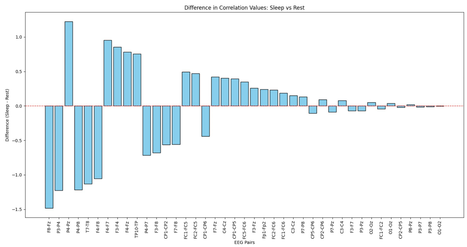
This step of data analysis focuses on comparing the cosine similarity between EEG channels during sleep and rest states. The top bar chart visualizes the channel-wise differences, highlighting which brain regions exhibit notable variations in activity patterns. The bottom chart aggregates these comparisons region-wise (e.g., Central, Occipital, Temporal), providing a high-level view of how different brain regions behave in sleep versus rest.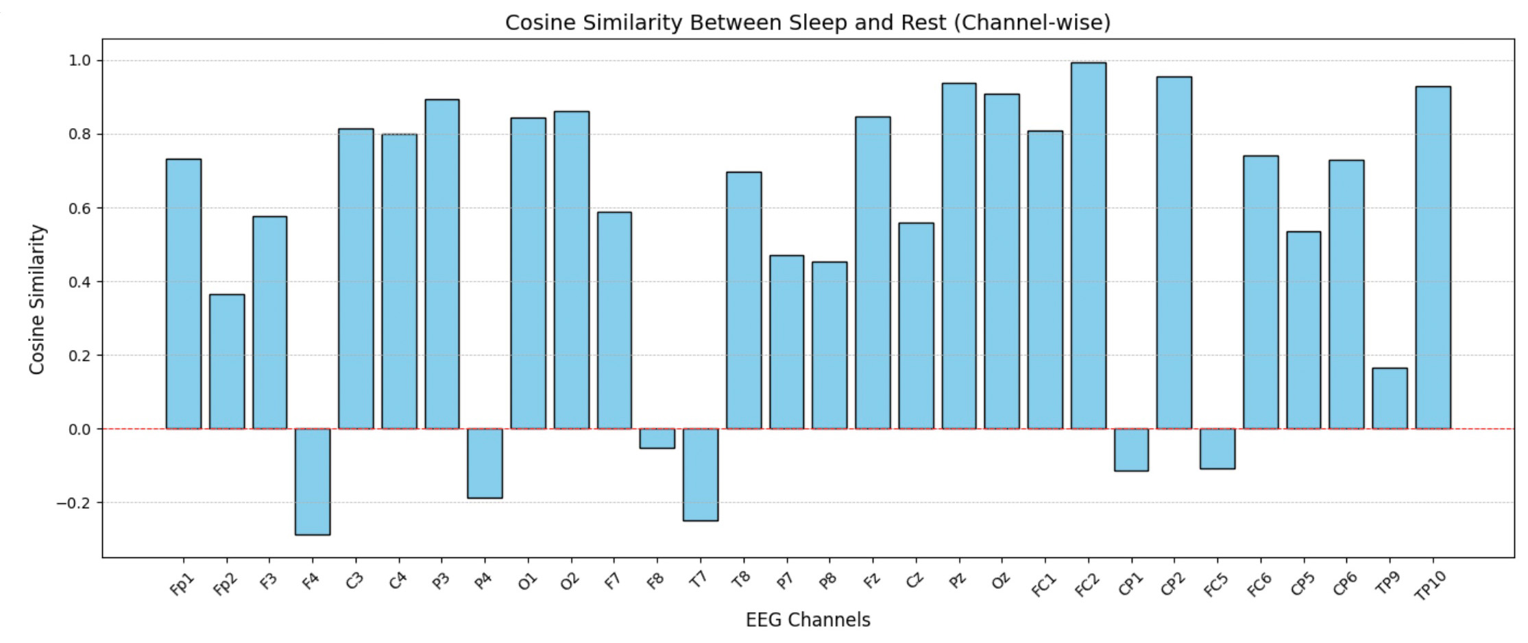
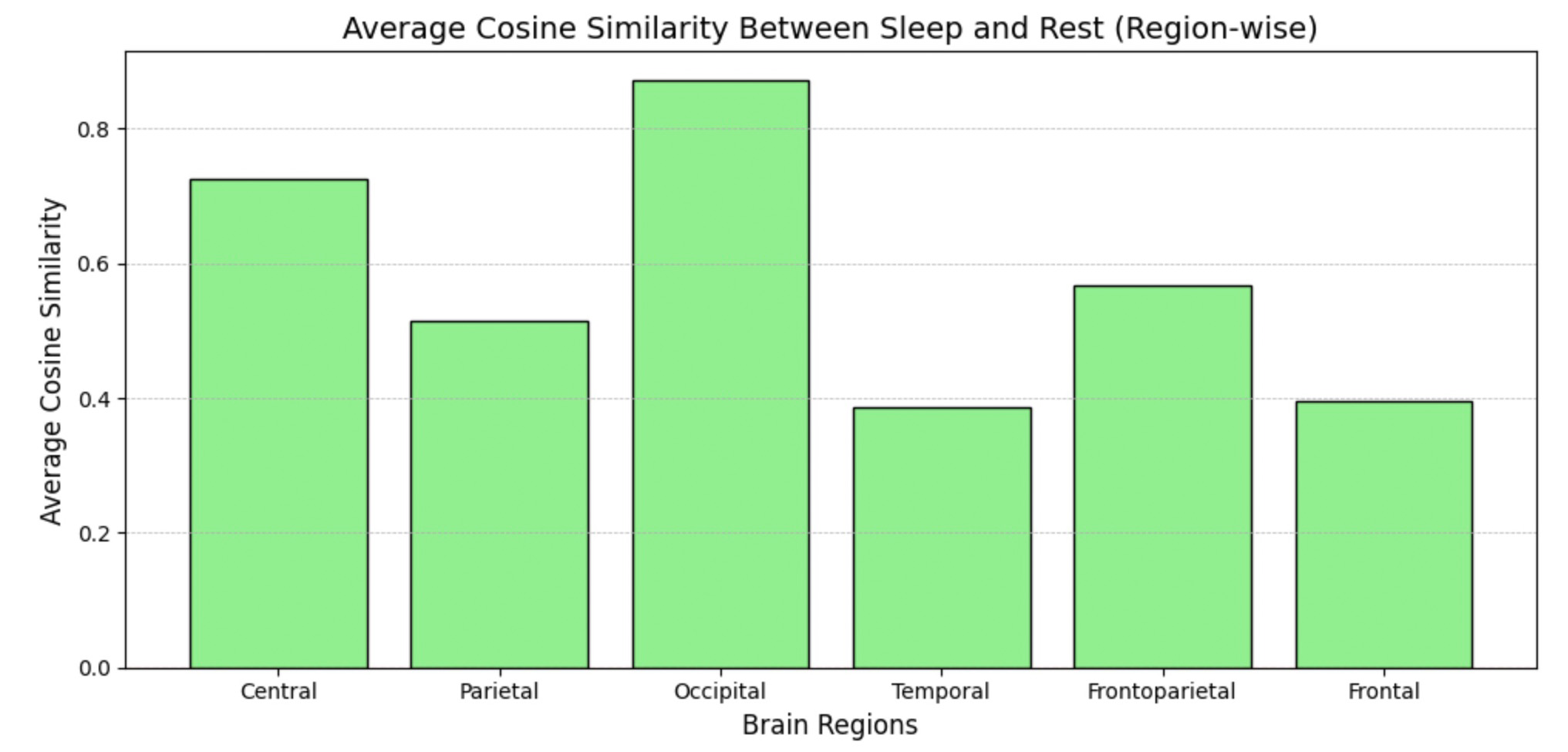 Since time measures in separate sections do not overlap, this comparison offers a broad overview, serving as a basis for more detailed studies on individual sessions.
Normalization and Preprocessing
In this step, we normalized the EEG data to ensure consistency across different sessions and reduce the impact of varying scales. The following processes were carried out:- Numerical Column Selection: Excluded the 'Time' column to focus only on the numerical EEG data for normalization.
-
Data Normalization:
Each feature was normalized using z-score normalization:
Normalized Value = (Value - Mean) / (Standard Deviation + 1e-5)
This ensures the data has a mean of 0 and a standard deviation of 1, improving the stability of subsequent analyses. -
Reintegrating the Time Column:
The 'Time' column was added back to the normalized dataset and renamed to
datefor easier readability and alignment with temporal analyses. -
String Representation for Dates:
Created a
dateStrcolumn by prefixing the time values with a tilde (~), providing a textual representation of the timestamps. -
Index Assignment:
Added a
rowIndexcolumn to assign a unique index to each row for tracking during further analysis.
eeg1_features = eeg1df.drop(columns=['Time'])
eeg2_features = eeg2df.drop(columns=['Time'])
eeg1 = (eeg1_features - eeg1_features.mean()) / (eeg1_features.std() + 1e-5)
eeg2 = (eeg2_features - eeg2_features.mean()) / (eeg2_features.std() + 1e-5)
eeg1['Time'] = eeg1df['Time']
eeg2['Time'] = eeg2df['Time']
eeg1=eeg1.rename(columns={'Time':'date'})
eeg2=eeg2.rename(columns={'Time':'date'})
eeg1['dateStr'] =  '~' + eeg1['date'].astype(str)
eeg2['dateStr'] =  '~' + eeg2['date'].astype(str)
eeg1['rowIndex'] = range(len(eeg1))
eeg2['rowIndex'] = range(len(eeg2))Channel Grouping by Brain Regions
To organize the EEG channels for our study, we grouped them based on their prefixes. This grouping helps us focus on specific brain regions for analysis and simplifies the selection process. Below are the steps and results of this process:-
Grouping Channels:
Each EEG channel was categorized by its prefix, which corresponds to the brain region it represents. Channels ending with
'z'were treated as central and grouped by removing the trailing'z'. For all other channels, their alphabetical prefix was used for grouping. - Code Implementation: The grouping was performed programmatically using a dictionary structure where the keys represent brain region prefixes, and the values contain the corresponding EEG channels.
from collections import defaultdict
channel_groups = defaultdict(list)
for channel in eeg1.columns:
    if channel.endswith('z'):
        prefix = channel[:-1]
    else:
        prefix = ''.join([char for char in channel if char.isalpha()])
    channel_groups[prefix].append(channel)
for group, channels in channel_groups.items():
    print(f"{group}: {channels}")
Grouped Channels
The resulting channel groups are as follows:- Fp: ['Fp1', 'Fp2']
- F: ['F3', 'F4', 'F7', 'F8', 'Fz']
- C: ['C3', 'C4', 'Cz']
- P: ['P3', 'P4', 'P7', 'P8', 'Pz']
- O: ['O1', 'O2', 'Oz']
- T: ['T7', 'T8']
- FC: ['FC1', 'FC2', 'FC5', 'FC6']
- CP: ['CP1', 'CP2', 'CP5', 'CP6']
- TP: ['TP9', 'TP10']
- EOG: ['EOG']
- ECG: ['ECG']
- Time: ['Time']
Computing Cosine Similarities Within EEG Channel Groups
As part of our EEG analysis, we calculated cosine similarities between channel pairs within the same group. This step focuses on understanding relationships between channels in specific brain regions. Below are the details of the process and implementation:Steps in Analysis
- Channel Grouping: EEG channels were grouped based on their prefixes, corresponding to specific brain regions. Channels ending with
'z'were adjusted by removing the trailing'z', and other channels were grouped by their letter prefixes. - Sorting Channels: Channels within each group were sorted alphabetically to ensure consistent pairwise comparisons.
- Cosine Similarity Calculation: Cosine similarities were computed for all possible pairs within each group using their numerical feature vectors.
- Sorting Results: The cosine similarity pairs were sorted alphabetically for easy interpretation and analysis.
from sklearn.metrics.pairwise import cosine_similarity
from collections import defaultdict
channel_groups = defaultdict(list)
for channel in eeg_df1_truncated.columns:
    if channel.endswith('z'):
        prefix = channel[:-1]
    else:
        prefix = ''.join([char for char in channel if char.isalpha()])
    channel_groups[prefix].append(channel)
cosine_similarities = {}
for group, channels in channel_groups.items():
    channels = sorted(channels)
    for i, channel1 in enumerate(channels):
        for channel2 in channels[i + 1:]:
            vector1 = eeg_df1_truncated[channel1].to_numpy().reshape(1, -1)
            vector2 = eeg_df1_truncated[channel2].to_numpy().reshape(1, -1)
            similarity = cosine_similarity(vector1, vector2)[0][0]
            cosine_similarities[f"{channel1}-{channel2}"] = similarity
sorted_cosine_similarities = dict(sorted(cosine_similarities.items()))- Cosine similarities provide insights into the relationships between EEG channels within the same brain region.
- The sorted similarity pairs offer a clear view of which channels are most or least correlated within each group.
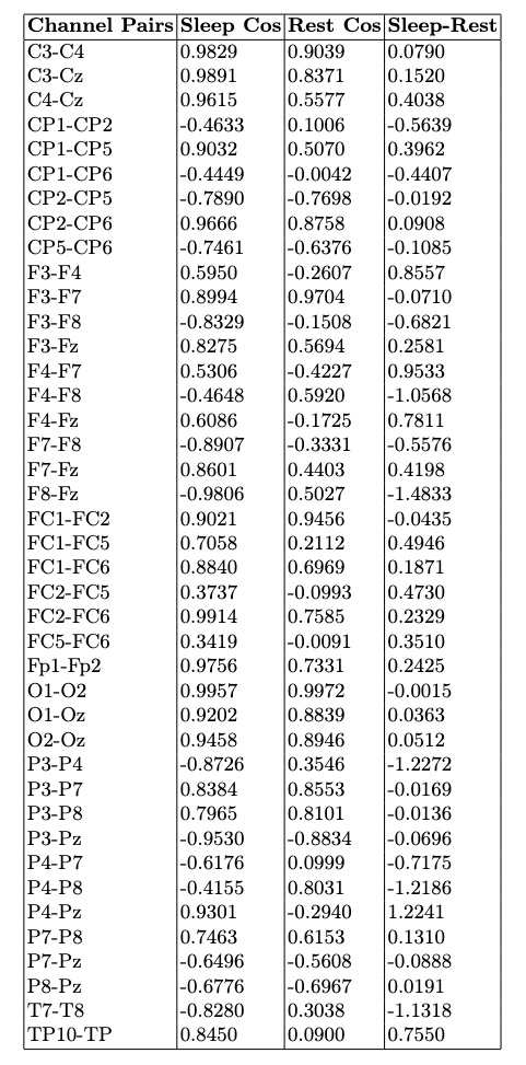
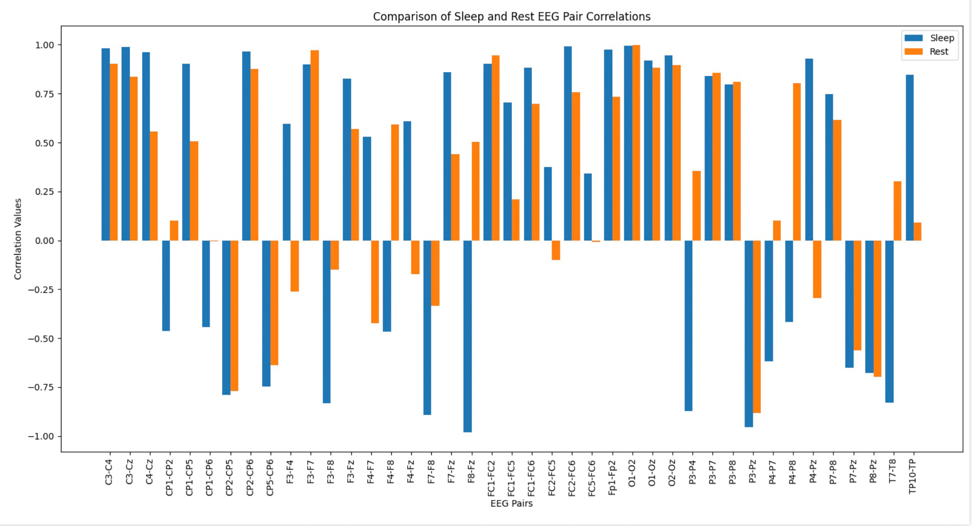
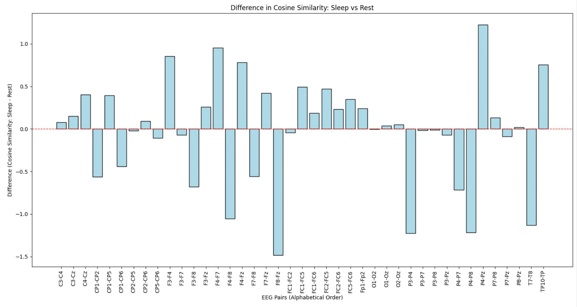
- Channel Pairs: EEG channel pairs analyzed for similarity.
- Sleep Cos: Cosine similarity during the sleep session.
- Rest Cos: Cosine similarity during the rest session.
- Sleep-Rest: Difference in similarity between sleep and rest, showing how connectivity changes across states.
 For our analysis, we selected the EEG channel pairs C4-Cz, F3-F4, and O1-O2. These pairs were chosen based on their relevance to brain region interactions and their notable differences in connectivity between sleep and rest states. These channels represent central, frontal, and occipital brain regions, providing a comprehensive view of neural activity across different areas of the brain.
Sliding Graph
This function,create_segments_df, is designed to process a time series DataFrame by creating overlapping segments for a specified column. It helps prepare data for sliding window analysis, which is essential for studying temporal patterns in EEG signals. Below is a high-level description of its workflow:
- Inputs: The function takes the following parameters:
df: The DataFrame containing the data.column_name: The column to segment.window_size: The size of each sliding window.shift: The step size for sliding the window.columnLabel: A label to annotate the segments.
- Process:
- Iterates over the DataFrame to extract overlapping windows of the specified size.
- Transposes each window to arrange its data as a single row for easier concatenation.
- Adds metadata to each segment, including:
start_date: The start time of the segment.rowIndex: The row index of the original DataFrame.theColumn: The name of the column being segmented.columnLabel: A label for the segment.
- Appends each processed segment to a list.
- Output: Combines all segments into a single DataFrame for downstream analysis.
def create_segments_df(df, column_name, window_size, shift,columnLabel):
    segments = []
    for i in range(0, len(df) - window_size + 1, shift):
        segment = df.loc[i:i + window_size - 1,
          [column_name]].reset_index(drop=True)
        segment = segment.T
        segment['start_date'] = df['date'][i]
        segment['rowIndex'] = df['rowIndex'][i]
        segment['theColumn'] = column_name
        segment['columnLabel'] = columnLabel
        segments.append(segment)
return pd.concat(segments, ignore_index=True)group_segments is designed to group smaller data segments into larger groups for graph-based analysis. This process is crucial for aggregating segments in sliding window studies, particularly for EEG analysis. Here’s a detailed explanation:
- Inputs: The function takes the following parameters:
segments_df: The DataFrame containing individual segments.group_size: The number of segments in each group.group_shift: The step size for sliding between groups.
- Process:
- Iterates over the DataFrame to extract overlapping groups of the specified size.
- Resets the index for each group to maintain consistent indexing.
- Adds a new column,
graphIndex, to assign a unique identifier to each group. - Appends each grouped segment to a list for aggregation.
- Increments the
group_indexafter each group to ensure unique identifiers.
- Output: Combines all grouped segments into a single DataFrame for further analysis or graph construction.
def group_segments(segments_df, group_size, group_shift):
    grouped_segments = []
    group_index = 0
    for i in range(0, len(segments_df) - group_size + 1, group_shift):
        group = segments_df.loc[i:i + group_size - 1].reset_index(drop=True)
        group['graphIndex'] = group_index
        grouped_segments.append(group)
        group_index += 1
    return pd.concat(grouped_segments, ignore_index=True)
Preprocessing and Sliding Window Preparation
Parameters for Sliding Window and Grouping: We defined the following parameters for creating sliding windows and grouping segments:- Window size (W): 32 data points per segment.
- Shift (S): 16 data points between segments.
- Group size (G): 32 segments per group.
- Group shift (Sg): 16 segments between groups.
window_size=32
shift=16
group_size=32
group_shift=16O1 and O2) for analysis and processed them as follows:
- Missing values were replaced with the mean of the respective column.
- Min-Max Scaling was applied to normalize the data for consistency across features.
O1 and O2), with each segment assigned a unique node index. Segments were then grouped into larger units for graph analysis.
Dataset Creation:
The grouped segments for both channels were concatenated into a single dataset. Each group was assigned a unique graph index, resulting in a dataset with 787 graph groups, ready for graph-based processing and analysis.
from sklearn.preprocessing import MinMaxScaler
pairColumns=['O1','O2']
col1 = pairColumns[0]
col2 = pairColumns[1]
scaler = MinMaxScaler()
fx_data=df
if col1 in fx_data.columns:
    fx_data[col1] = fx_data[col1].fillna(fx_data[col1].mean())
    fx_data[col1] = scaler.fit_transform(fx_data[[col1]])
if col2 in fx_data.columns:
    fx_data[col2] = fx_data[col2].fillna(fx_data[col2].mean())
    fx_data[col2] = scaler.fit_transform(fx_data[[col2]])
columnLabel=0
segments1 = create_segments_df(df, col1, window_size, shift, columnLabel)
columnLabel=1
segments2 = create_segments_df(df, col2, window_size, shift, columnLabel)
segments1['nodeIndex']=segments1.index
segments2['nodeIndex']=segments2.index
grouped_segments1 = group_segments(segments1, group_size, group_shift)
grouped_segments2 = group_segments(segments2, group_size, group_shift)
dataSet= pd.concat([grouped_segments1, grouped_segments2], ignore_index=True)
graphMax = dataSet['graphIndex'].max()
graphMax
787
Sliding Window Graph as Input for GNN Graph Classification
In this stage of our analysis, we prepared sliding window graphs as input for a Graph Neural Network (GNN) classification task. Below is a high-level description of the process: Process Overview: We iteratively constructed graphs for EEG data using the predefined sliding windows and grouped segments. Each graph corresponds to a unique segment of the EEG data, capturing temporal relationships within the window. For each graph:- Features (
x): Derived from EEG signal values within the segment, including the average of node features to enhance representation. - Edges (
edge_index): Created based on cosine similarity between node pairs, using a threshold (cos > 0.9) to establish connections between nodes. - Labels (
y): Assigned based on the channel being analyzed (e.g.,O1orO2).
- DatasetTest: Contains graphs prepared for evaluation.
- DatasetModel: Contains graphs ready for training the GNN model.
DataLoader for efficient batch processing during model training and evaluation.
Outcome:
The constructed sliding window graphs provide a structured and efficient way to capture temporal EEG patterns for graph-based classification. This approach highlights the power of combining sliding window analysis with GNNs to study EEG signals.
from torch_geometric.loader import DataLoader
cos=0.9
datasetTest=list()
datasetModel=list()
cosPairsUnion=pd.DataFrame()
for label in range(0,2):
  column=pairColumns[label]
  for graphIdx in range(0, graphMax):
    data1=dataSet[(dataSet['graphIndex']==graphIdx)
      & (dataSet['theColumn']==column)]
    values1=data1.iloc[:,:-7]
    fXValues1= values1.fillna(0).values.astype(float)
    fXValuesPT1=torch.from_numpy(fXValues1)
    fXValuesPT1avg=torch.mean(fXValuesPT1,dim=0).view(1,-1)
    fXValuesPT1union=torch.cat((fXValuesPT1,fXValuesPT1avg),dim=0)
    cosine_scores1 = pytorch_cos_sim(fXValuesPT1, fXValuesPT1)
    cosPairs1=[]
    score0=cosine_scores1[0][0].detach().numpy()
    for i in range(group_size):
      date1=data1.iloc[i]['start_date']
      datasetIdx=data1.iloc[i]['datasetIdx']
      cosPairs1.append({'cos':score0, 'graphIdx':graphIdx,
                        'label':label,'theColumn':column,
                        'k1':i, 'k2':window_size,
                        'date1':date1,
                        'date2':'XXX','datasetIdx': datasetIdx,
                        'score': score0})
      for j in range(group_size):
        if i<j:
          score=cosine_scores1[i][j].detach().numpy()
          if score>cos:
            date2=data1.iloc[j]['start_date']
            datasetIdx=data1.iloc[i]['datasetIdx']
            cosPairs1.append({'cos':cos, 'graphIdx':graphIdx,
                              'cos':score0, 'graphIdx':graphIdx,
                              'label':label,'theColumn':column,
                              'k1':i,
                              'k2':j,
                              'date1':date1,
                              'date2':date2,
                              'datasetIdx': datasetIdx,
                              'score': score})
    dfCosPairs1=pd.DataFrame(cosPairs1)
    edge1=torch.tensor(dfCosPairs1[['k1',	'k2']].T.values)
    dataset1 = Data(edge_index=edge1)
    dataset1.y=torch.tensor([label])
    dataset1.x=fXValuesPT1union
    datasetTest.append(dataset1)
    loader = DataLoader(datasetTest, batch_size=32)
    loader = DataLoader(datasetModel, batch_size=32)
    cosPairsUnion = pd.concat([cosPairsUnion, dfCosPairs1], ignore_index=True)
GNN Graph Classification: Model Training.
To classify EEG data using a graph neural network (GNN), we implemented a training pipeline that incorporates data splitting, model definition, and training steps. Below is an overview of the process:from sklearn.model_selection import train_test_split
from torch_geometric.loader import DataLoader
test_size = 0.17
train_dataset, test_dataset =
train_test_split(graphInput, test_size=test_size, random_state=42)
train_loader = DataLoader(train_dataset, batch_size=16, shuffle=True)
test_loader = DataLoader(test_dataset, batch_size=16, shuffle=False)- Node Embedding Steps: Three graph convolutional layers process node-level information.
- Graph Embedding Step: A global mean pooling layer aggregates node-level embeddings into graph-level embeddings.
- Classification Step: A fully connected layer classifies graphs into two categories.
from torch.nn import Linear
import torch.nn.functional as F
from torch_geometric.nn import GCNConv
from torch_geometric.nn import global_mean_pool
class GCN(torch.nn.Module):
    def __init__(self, hidden_channels):
        super(GCN, self).__init__()
        torch.manual_seed(12345)
        self.conv1 = GCNConv(window_size, hidden_channels)
        self.conv2 = GCNConv(hidden_channels, hidden_channels)
        self.conv3 = GCNConv(hidden_channels, hidden_channels)
        self.lin = Linear(hidden_channels, 2)
    def forward(self, x, edge_index, batch, return_graph_embedding=False):
        x = self.conv1(x, edge_index)
        x = x.relu()
        x = self.conv2(x, edge_index)
        x = x.relu()
        x = self.conv3(x, edge_index)
        graph_embedding = global_mean_pool(x, batch)
        if return_graph_embedding:
            return graph_embedding
        x = F.dropout(graph_embedding, p=0.3, training=self.training)
        x = self.lin(x)
        return x
model = GCN(hidden_channels=16)Model Training and Evaluation
The training and evaluation process for the GNN model involves key steps to optimize the parameters and assess performance. Below is an overview of the methodology: Training Process:- Perform a single forward pass over batches in the training dataset.
- Compute the loss using the cross-entropy loss function.
- Derive gradients using backpropagation.
- Update model parameters based on the computed gradients.
- Clear gradients after each step to prevent accumulation.
- Iterate over the test dataset in batches.
- Perform forward passes to compute predictions.
- Use the class with the highest probability as the predicted label.
- Compare predictions with ground-truth labels to compute the accuracy.
- Return the ratio of correct predictions as the evaluation metric.
from IPython.display import Javascript
display(Javascript('''google.colab.output.setIframeHeight(0, true, {maxHeight: 300})'''))
model = GCN(hidden_channels=16)
optimizer = torch.optim.Adam(model.parameters(), lr=0.001)
criterion = torch.nn.CrossEntropyLoss()
def train():
    model.train()
    for data in train_loader:
         out = model(data.x.float(), data.edge_index, data.batch)
         loss = criterion(out, data.y)
         loss.backward()
         optimizer.step()
         optimizer.zero_grad()
def test(loader):
     model.eval()
     correct = 0
     for data in loader:
         out = model(data.x.float(), data.edge_index, data.batch)
         pred = out.argmax(dim=1)
         correct += int((pred == data.y).sum())
return correct / len(loader.dataset) for epoch in range(1, 17):
train()
train_acc = test(train_loader)
test_acc = test(test_loader)
print(f'Epoch: {epoch:03d},
Train Acc: {train_acc:.4f},
Test Acc: {test_acc:.4f}')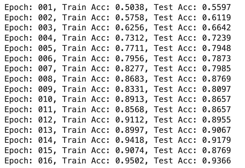
- Training Accuracy: Indicates the model's ability to learn patterns from the training dataset. Accuracy steadily increased across epochs, reaching a peak of 0.9502.
- Test Accuracy: Reflects the model's performance on unseen test data, gradually improving and achieving a high value of 0.9366 by the final epoch.
Analysis of Cosine Similarity and GNN Performance for Selected EEG Pairs
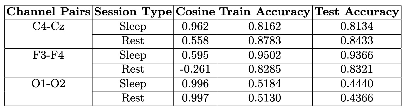 This table presents cosine similarity values and GNN Graph Classification performance for selected EEG channel pairs across sleep and rest states, offering insights into connectivity patterns and classification accuracy.
- Cosine Similarity & Channel Interactions:
- F3-F4 (Frontal Lobe): Moderate similarity in both states with the highest training and test accuracy, indicating strong differentiation between sleep and rest.
- C4-Cz (Central Region): Higher similarity during sleep, suggesting stronger functional connectivity in this state. However, its stable patterns across conditions resulted in moderate classification accuracy.
- O1-O2 (Occipital Lobe): Consistently high similarity across both states, limiting classification performance due to minimal variation.
- Brain Regions & Functional Roles:
- Frontal Activity (F3-F4): Notable differences in similarity between sleep and rest align with the frontal lobe’s role in cognitive processing, which decreases during sleep.
- Visual Processing (O1-O2): The occipital lobe pair maintained stable interactions across states, reflecting consistent neural activity in visual regions.
- Model Performance & Interpretation:
- Training Accuracy: The GNN effectively learned EEG patterns, with F3-F4 achieving the highest accuracy, reinforcing its distinct connectivity changes across states.
- Test Accuracy: Performance varied across pairs; F3-F4 demonstrated strong generalization, while others showed moderate accuracy shifts.
- High Similarity & Lower Accuracy: While strong cosine similarity suggests stable EEG interactions, it can reduce variability needed for classification. This is evident in O1-O2, where consistently high similarity limited the model’s ability to distinguish between sleep and rest.
Note on O1-O2 Analysis
Although O1-O2 was initially included as part of the analysis, its results have been excluded from the figures and detailed discussion due to the very low model training and testing accuracy observed for this channel pair. This suggests that the model failed to capture meaningful patterns or dynamics for O1-O2, likely due to insufficient signal quality or inherent limitations in the data for this pair.Model Results Interpretation
The results interpretation phase analyzed the predictions and embeddings from the GNN Graph Classification model. A softmax function transformed the model’s outputs into probabilities, making classification predictions more interpretable. This process helped identify the most likely labels for each graph. Process:- Softmax Transformation: The raw outputs of the GNN model were passed through a softmax function to convert them into probability distributions over the possible classes.
- Prediction Extraction: The predicted labels for each graph were determined by identifying the class with the highest probability.
- Graph Embeddings: The GNN model also generated graph-level embeddings for each graph, providing a compact vector representation of the patterns captured within the graph.
- Data Storage: These embeddings, along with the predicted labels and probabilities, were stored in a structured DataFrame for further analysis and visualization.
softmax = torch.nn.Softmax(dim = 1)
graphUnion=[]
for g in range(graphCount):
  label=dataset[g].y[0].detach().numpy()
  out = model(dataset[g].x.float(), dataset[g].edge_index, dataset[g].batch, return_graph_embedding=True)
  output = softmax(out)[0].detach().numpy()
  pred = out.argmax(dim=1).detach().numpy()
graphUnion.append({'index':g,'vector': out.detach().numpy()})graphUnion_df=pd.DataFrame(graphUnion)
graphUnion_df.tail()
index vector
1569 1569 [[0.17810732, -0.19235992, -0.16263075, -0.167...
1570 1570 [[0.2913107, -0.073132396, -0.09579194, -0.039...
1571 1571 [[0.030929727, -0.10722159, -0.040990006, -0.0...
1572 1572 [[0.3690454, -0.014458519, 0.03268631, 0.04397...
1573 1573 [[0.123519175, -0.23811509, -0.22812074, -0.16.Cosine Similarity Analysis for Graph Embeddings
This step evaluates the similarity between pre-final embedding vectors generated by the GNN model for sliding window graphs. By calculating cosine similarity, we gain insights into the relationships and connectivity patterns captured by the model. Key Steps:- Graph Embedding Vectors: Each graph is represented by a vector derived from the GNN's pre-final embedding layer, summarizing temporal and spatial relationships within the EEG signal.
- Middle Point Calculation: For each pair of graph embeddings, the middle point between their corresponding time windows is calculated to align temporal information with similarity analysis.
- Cosine Similarity: Cosine similarity is computed between graph embedding vectors to quantify the relationship between graphs. This metric reveals how closely related the patterns in the two time segments are.
- Result Compilation: The results include cosine similarity scores and metadata like the middle point of time windows. These scores provide a basis for exploring the relationships in EEG data.
cosine_sim_pairs = []
for i in range(len(graphList_1)):
    datasetIdx_0=graphList_0['datasetIdx'][i]
    datasetIdx_1=graphList_1['datasetIdx'][i]
    min = graphList_0['min'][i]
    max = graphList_1['max'][i]
    middle_point = (min+max)/2
    # cos_sim_value = cos_sim(datasetIdx_0, datasetIdx_1).numpy().flatten
    vector_0 = torch.tensor(graphUnion_df['vector'][datasetIdx_0])
    vector_1 = torch.tensor(graphUnion_df['vector'][datasetIdx_1])
    cos_sim_value = cos_sim(vector_0, vector_1).numpy().flatten()[0]
    cosine_sim_pairs.append({
            'middle_point':middle_point,
            'cos': cos_sim_value
})Analysis of Embedded Graphs: Statistics
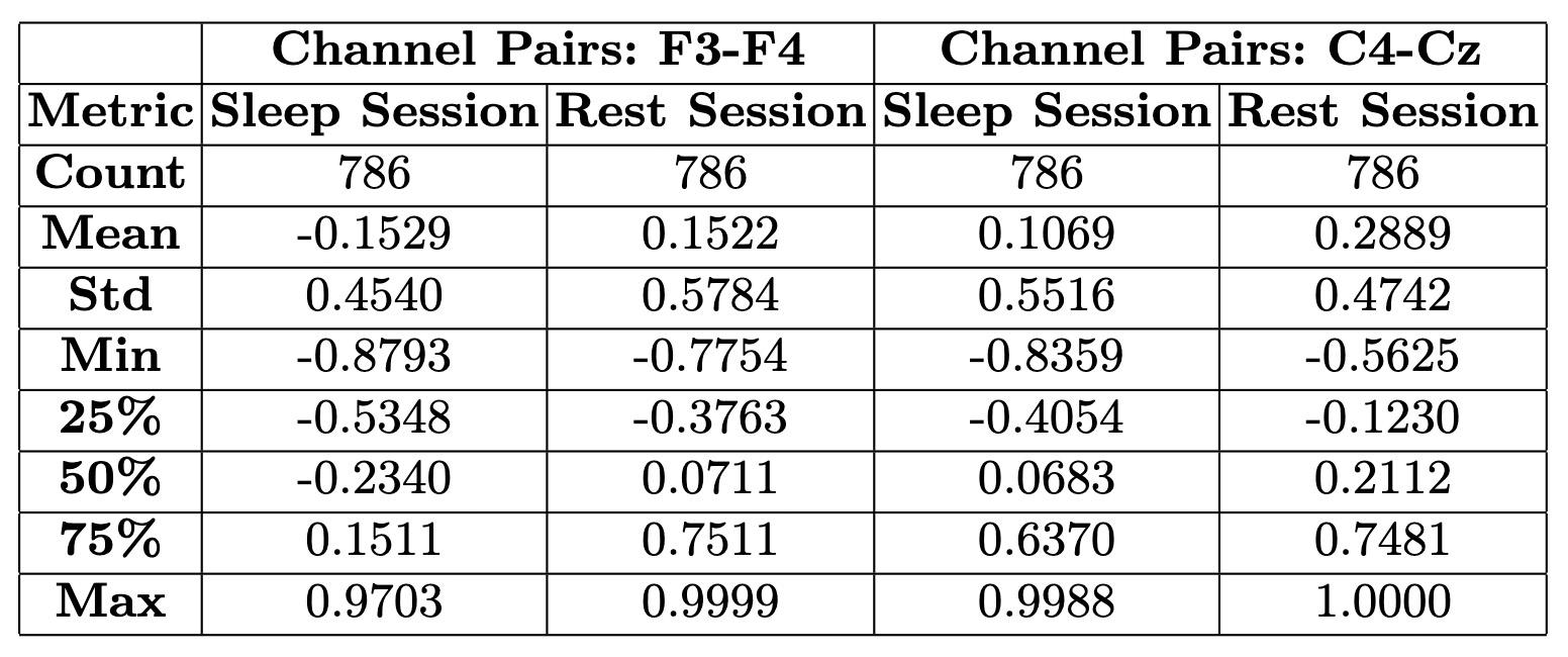
Temporal Analysis of Connectivity Within Sleep and Rest
Understanding how connectivity evolves within each state requires a detailed temporal analysis. While statistical comparisons provide an overview of differences between sleep and rest, examining connectivity patterns over time within each session offers deeper insights. Figures below present a time-resolved views of cosine similarities for F3-F4 and C4-Cz, capturing fluctuations in connectivity as they unfold. This approach helps identify transient changes, sustained trends, and potential transitions in neural activity, providing a more nuanced understanding of brain dynamics in sleep and rest.Transforming Time Points
First, we converted the middle points of each sliding window into minutes and seconds to provide a clear temporal context. This was achieved by calculating the integer division and modulo of the middle points by 60 to derive minutes and seconds, respectively. These were then formatted into readable time labels (e.g., "12m 34.5s") for enhanced interpretability in our plots.cosine_sim_pairs_df['minutes'] = cosine_sim_pairs_df['middle_point'] // 60
cosine_sim_pairs_df['seconds'] = cosine_sim_pairs_df['middle_point'] % 60
cosine_sim_pairs_df['time_label'] = cosine_sim_pairs_df['minutes']
.astype(int).astype(str) + 'm ' + cosine_sim_pairs_df['seconds']
.round(3).astype(str) + 's'Smoothing Cosine Similarity Values
Next, to reduce noise and highlight meaningful trends, we applied a Gaussian smoothing filter to the cosine similarity values. This technique helps clarify patterns by averaging adjacent points in the time series, resulting in smoother curves that better represent the underlying data.Creating the Plot
The smoothed cosine similarity values for both channel pairs were plotted against their corresponding time points. Key details of the plot include:- X-axis: Time in minutes and seconds, with custom ticks to reduce clutter, ensuring a clear and focused visualization.
- Y-axis: Cosine similarity values, representing the strength of connectivity between the selected EEG channels.
- Curves: Separate lines for each channel pair (F3-F4 and C4-Cz) to allow for direct comparison of their temporal dynamics.
Insights and Observations
The resulting plot showcases how connectivity between specific brain regions changes over time. The F3-F4 pair, for instance, might exhibit distinct patterns compared to C4-Cz, reflecting differences in activity across these regions. This visualization provides a foundation for deeper analyses, such as correlating these dynamics with behavioral or physiological states.Technical Details
The plot was created using Python libraries, includingmatplotlib for visualization and scipy.ndimage for smoothing. The data preparation involved grouping cosine similarity values, aligning them temporally, and ensuring consistency in the time axis for both channel pairs. This ensures an accurate and visually compelling comparison of the EEG data's temporal features.
By transforming, smoothing, and plotting the cosine similarity values, this analysis offers a detailed view of temporal connectivity dynamics in EEG data. It provides a vital step in understanding the intricate relationships between brain regions and their changes across different states, such as sleep and rest.
import matplotlib.pyplot as plt
from scipy.ndimage import gaussian_filter1d
cos_smoothed_sleep = gaussian_filter1d(cosine_sim_pairs_df1['cos'], sigma=2)
cos_smoothed_rest = gaussian_filter1d(cosine_sim_pairs_df2['cos'], sigma=2)
time_labels = cosine_sim_pairs_df1['time_label']
step_size = 60
x_ticks = cosine_sim_pairs_df1['middle_point'][::step_size]
x_labels = [f"{int(m)}:{s:.1f}" for m,
  s in cosine_sim_pairs_df1[['minutes', 'seconds']].iloc[::step_size].values]
plt.figure(figsize=(12, 6))
plt.plot(
    cosine_sim_pairs_df1['middle_point'], cos_smoothed_sleep,
    label='F3-F4', color='brown', linewidth=1.5
)
plt.plot(
    cosine_sim_pairs_df2['middle_point'], cos_smoothed_rest,
    label='C4-Cz', color='green', linewidth=1.5
)
plt.xticks(x_ticks, x_labels, rotation=15, fontsize=10)
plt.xlabel('Time (minutes:seconds)', fontsize=12)
plt.ylabel('Cosine Similarity', fontsize=12)
plt.title('Cosine Similarity at Rest Time: F3-F4 vs. C4-Cz', fontsize=14)
plt.grid(alpha=0.3)
plt.legend()
plt.show()
Cosine Similarity at Sleep Time: F3-F4 vs. C4-Cz
This figure illustrates the temporal dynamics of cosine similarity for two EEG channel pairs, F3-F4 and C4-Cz, during sleep. The x-axis represents time in minutes and seconds, while the y-axis shows the cosine similarity values. The red line corresponds to the F3-F4 channel pair, and the green line corresponds to the C4-Cz channel pair. The fluctuations in similarity values over time highlight differences in connectivity between these brain regions during sleep. This visualization offers a detailed view of how specific brain areas interact dynamically during sleep, capturing subtle connectivity changes.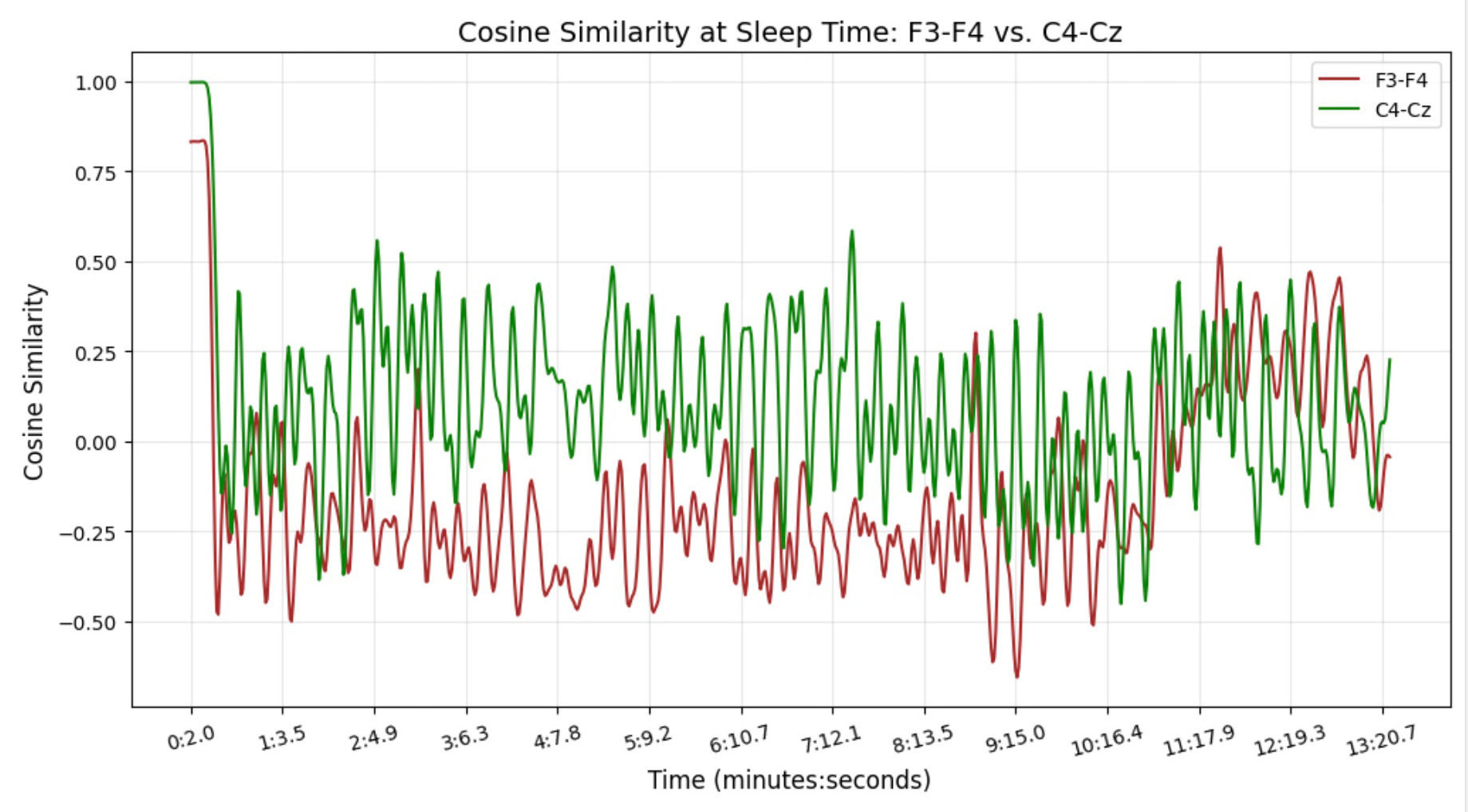
Cosine Similarity at Rest Time: F3-F4 vs. C4-Cz
This figure depicts the cosine similarity for the same EEG channel pairs, F3-F4 and C4-Cz, during rest. Similar to the sleep plot, the x-axis indicates time in minutes and seconds, and the y-axis represents cosine similarity values. The trends for F3-F4 (red) and C4-Cz (green) reveal distinct patterns of connectivity during rest, differing from the sleep state. These patterns reflect how brain activity and connectivity are modulated across different states.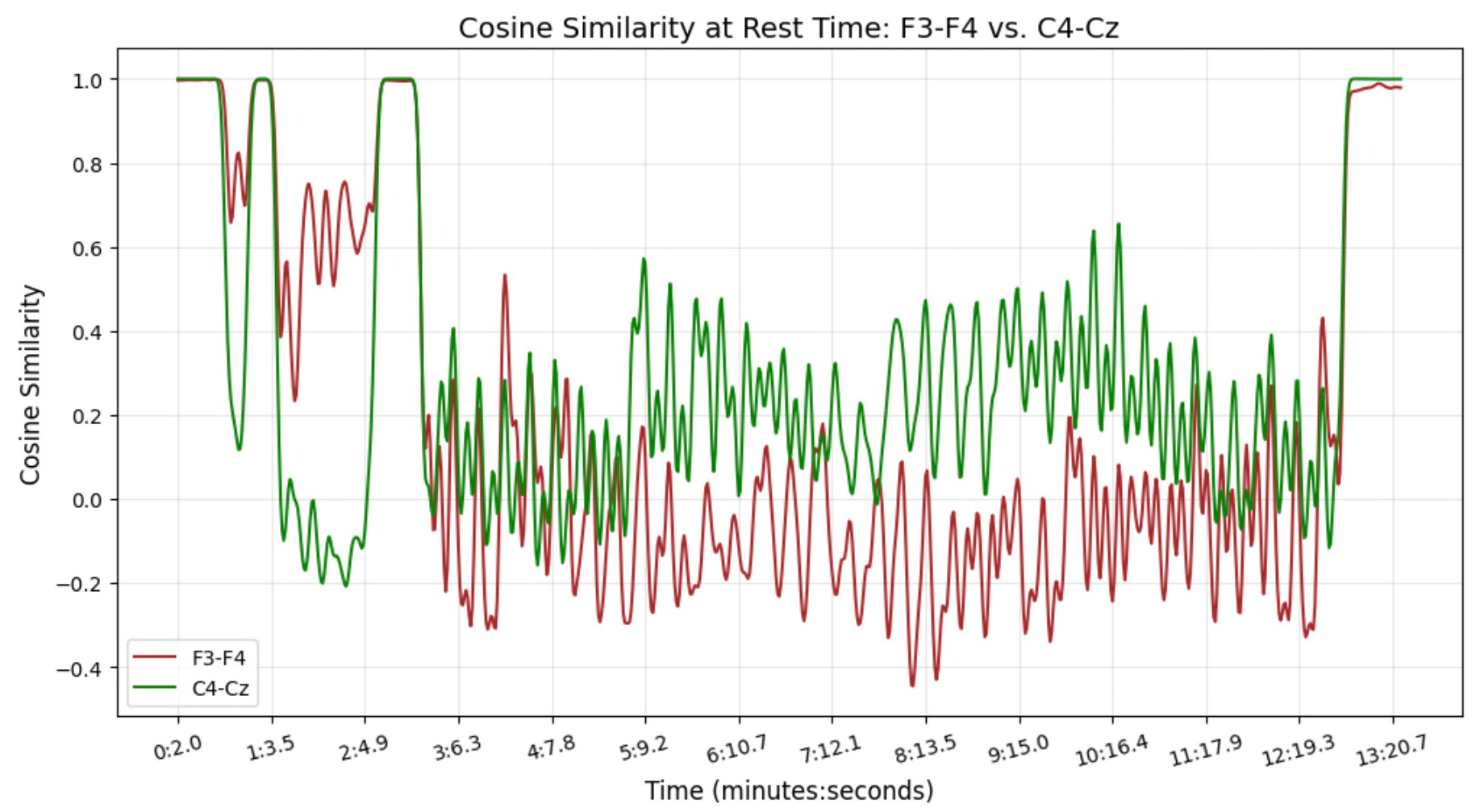
Conclusion
This study explores how sliding graph neural networks can help analyze EEG time series, capturing shifting connectivity patterns in the brain. By transforming EEG signals into overlapping graphs, GNN Graph Classification not only tracks how brain activity changes over time but also provides deeper insights into neural interactions beyond simple classification.
Our findings highlight clear differences between sleep and rest, especially in the frontal (F3-F4) and central (C4-Cz) regions. Cosine similarity analysis shows that while C4-Cz remains strongly connected during rest, F3-F4 shifts more between states, reflecting how different brain areas behave across conditions.
Bringing neuroscience and graph theory together opens exciting possibilities. Sliding graphs give neuroscientists a fresh way to uncover EEG patterns that might go unnoticed with traditional methods, while graph-based techniques gain new applications in sleep research. This collaboration isn’t just about analyzing data—it’s about connecting disciplines and discovering new ways to study the brain.
Beyond EEG, GNN Sliding Graph Classification has potential in many fields, from tracking climate trends to understanding financial markets. With opportunities to scale, improve interpretability, and tackle real-world challenges, this approach could offer fresh insights into complex systems far beyond neuroscience.