Sliding Window Graph in GNN Graph Classification

The use of Graph Neural Networks (GNNs) in time series analysis represents a rising field of study, particularly in the context of GNN Graph Classification, a technique traditionally applied in disciplines such as biology and chemistry. Our research repurposes GNN Graph Classification for the analysis of time series climate data, focusing on two distinct methodologies: the city-graph method, which effectively captures static temporal snapshots, and the sliding window graph method, adept at tracking dynamic temporal changes. This innovative application of GNN Graph Classification within time series data enables the uncovering of nuanced data trends.

We demonstrate how GNNs can construct meaningful graphs from time series data, showcasing their versatility across different analytical contexts. A key finding is GNNs’ adeptness at adapting to changes in graph structure, which significantly improves outlier detection. This enhances our understanding of climate patterns and suggests broader applications of GNN Graph Classification in analyzing complex data systems beyond traditional time series analysis. Our research seeks to fill a gap in current studies by providing an examination of GNNs in climate change analysis, highlighting the potential of these methods in capturing and interpreting intricate data trends.

Conference Presentation: ICMLT 2024

This study was presented at the International Conference on Machine Learning Technologies (ICMLT) and is included in the proceedings.

In our research, we combined and compared two methods for analyzing time series climate data using Graph Neural Networks (GNNs). Our previous study, “GNN Graph Classification for Climate Change Patterns: Graph Neural Network (GNN) Graph Classification - A Novel Method for Analyzing Time Series Data”, introduced the city-graph method, which captures static temporal snapshots to sort climate data into ‘stable’ and ‘unstable’ categories. In this post, we focus on our new technique: the sliding window graph method. This approach breaks down time series data into overlapping sections to capture specific time-related features. These sections are then used to create graphs, providing a new way to understand short-term changes in climate patterns.

Introduction

In 2012, deep learning and knowledge graphs took a big leap forward in data analysis and machine learning. AlexNet, a new type of Convolutional Neural Network (CNN) for image classification, showed much better results than older methods. Around the same time, Google introduced knowledge graphs, which improved how data is integrated and managed.

However, CNNs struggled with graph-structured data, and graph techniques lacked deep learning’s ability to recognize patterns. This changed with the arrival of Graph Neural Networks (GNNs). GNNs combined deep learning with graph data processing, making it easier to analyze graph-structured data.

GNN models are designed specifically for graph data. They use geometric relationships and combine node features with graph structure. This makes them very useful for tasks like node classification, link prediction, and graph classification. GNN Graph Classification models, which have been used in areas like chemistry and medicine, classify entire graphs based on their structure and features.

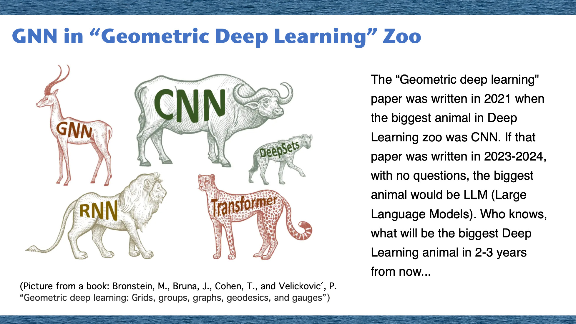
In 2021, the “Geometric Deep Learning” paper was written when Convolutional Neural Networks (CNNs) were the dominant models in the deep learning landscape. If the paper were written in 2023-2024, Large Language Models (LLMs) would undoubtedly be considered the leading technology. The field of deep learning is rapidly evolving, and it remains to be seen what new advancements and models will emerge as the “biggest animals” in the next 2-3 years.

In this study, we expand on our previous research using Graph Neural Network (GNN) models to analyze climate data. Our earlier method categorized climate time series data into ‘stable’ and ‘unstable’ to identify unusual patterns in climate change.

Now, we introduce the sliding window graph method, which breaks down time series data into overlapping sections to capture specific time-related features. This approach creates graphs from these sections, offering a new perspective on short-term climate changes.

Our previous study used a city-graph method, where nodes represent city-year combinations with daily temperature vectors as features. The new sliding window method compares identical dates across different cities and years, helping us understand global climate trends.

Our research aims to explore the potential of GNN graph classification in identifying and interpreting global climate dynamics, providing valuable insights into seasonal changes and long-term shifts in climate.

Methods

Graph Construction Methods

In our study, we explore two different methods for constructing graphs from climate data: the City-Graph Method and the Sliding Window Method.

City-Graph Method:

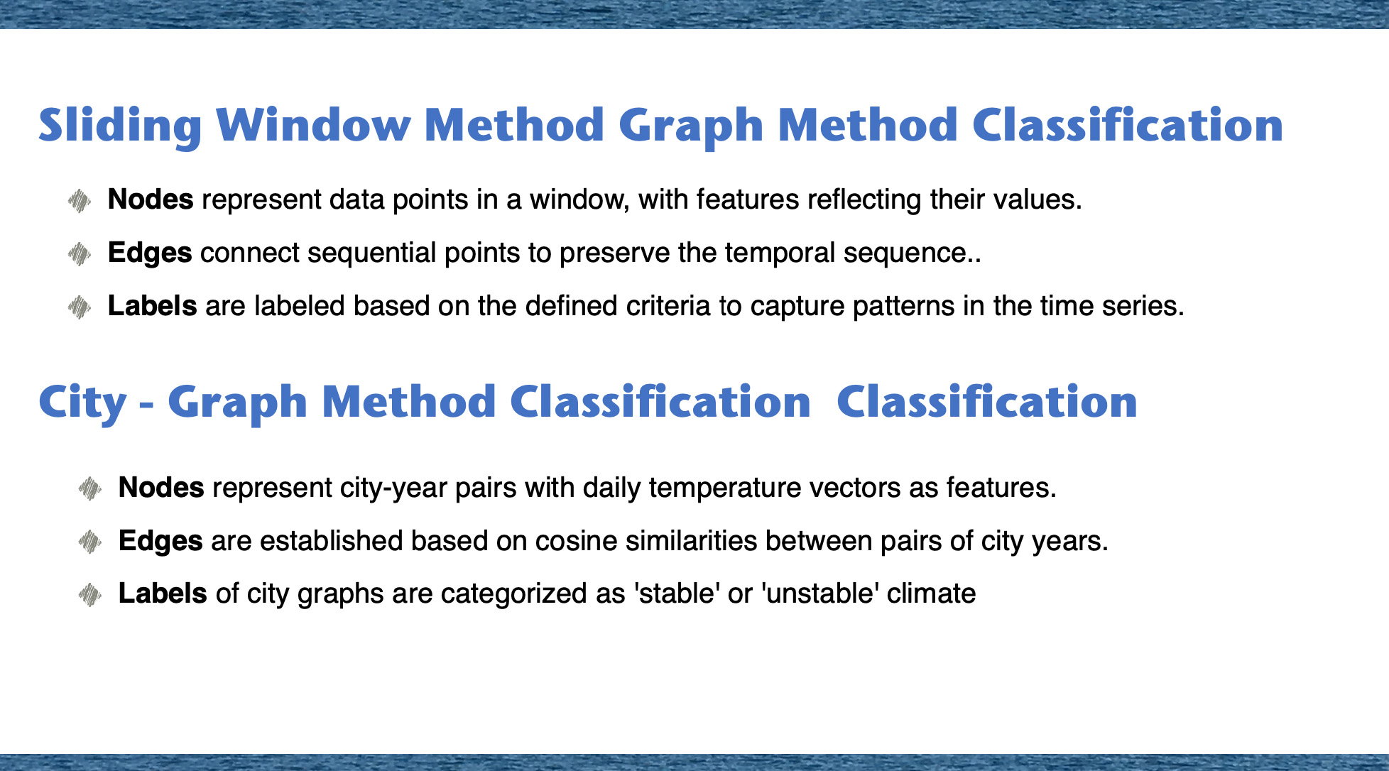
• Creating graphs where nodes represent city-year pairs.
• Features are daily temperature vectors for each city-year.
• Edges are established based on cosine similarities between the temperature vectors of different city-years.
• Categorizes city graphs into 'stable' or 'unstable' climates based on their temperature patterns over time.

Sliding Window Method:

• Constructing graphs by breaking down time series data into overlapping sections.
• Nodes represent data points within a sliding window, with features reflecting their values.
• Edges connect sequential points to maintain the temporal sequence.
• Labels are assigned to capture patterns within the time series.

Common Pipeline

While the graph construction methods differ, both follow a common pipeline for GNN Graph Classification:

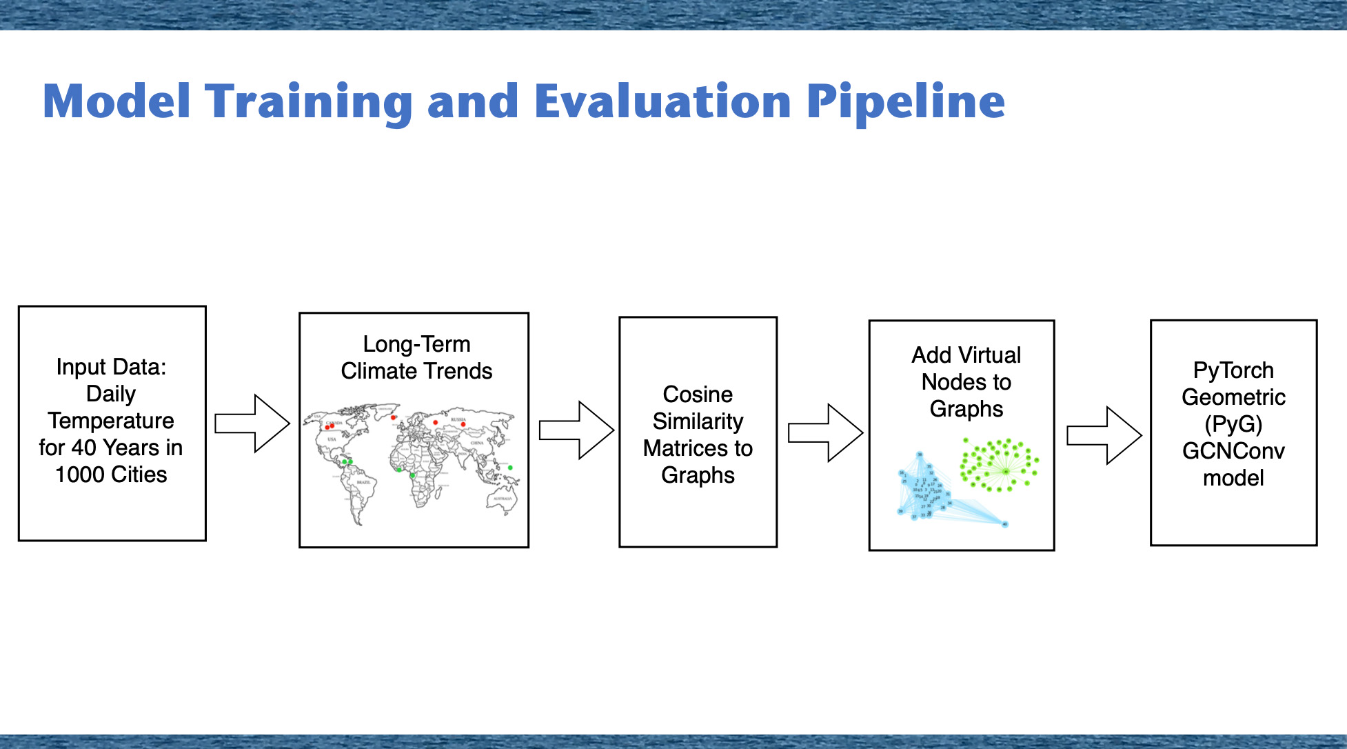
• Data Input: daily temperature data for 1000 populous cities over 40 years.
• Climate Trends as 'stable' or 'unstable'.
• Graph Construction:
  • City-Graph Method.
  • Sliding Window Method.
• Virtual Nodes: to act as central hubs in small graphs, tuning the models for better accuracy..
• GNN Model Application: use GNN model to classify graphs based on patterns.

Methodology for Sliding Window Graph Construction

Our approach uses Graph Neural Networks (GNNs) combined with a sliding window technique to analyze time series data. Here’s an overview of the process:

Data to Graph Transformation

We segment time series data into smaller graphs using a sliding window, which captures local temporal patterns. Each time segment forms a unique graph.

Graph Creation

In these graphs, nodes represent data points within the window, with features reflecting their values. Edges connect these sequential points to maintain the temporal order.

Crucial Parameters

The window size (W) and overlap (shift size S) are important as they determine how the data is segmented and analyzed. Edge definitions within the graphs are tailored to the specifics of the time series data, helping to detect patterns.

Node Calculation

For a dataset with N data points, we apply a sliding window of size W with a shift of S to create nodes. The number of nodes, N_nodes, is calculated as: $N_{\mathrm{nodes}}=\lfloor \frac{N-W}{S}\rfloor +1$

Graph Calculation

With the nodes determined, we construct graphs, each comprising G nodes, with a shift of S_g between successive graphs. The number of graphs, N_graphs, is calculated by: $N_{\mathrm{graphs}}=\lfloor \frac{N_{\mathrm{nodes}}-G}{S_g}\rfloor +1$

This method allows us to analyze time series data effectively by capturing both local and global patterns, providing valuable insights into temporal dynamics.

Model Training

Our methodology involves processing both city-centric and sliding window graphs. We start by generating cosine similarity matrices from time series data, which are then converted into graph adjacency matrices. This process includes creating edges for vector pairs with cosine values above a set threshold and adding a virtual node to ensure network connectivity, a critical step for preparing the graph structure.

For graph classification tasks, we use the GCNConv model from the PyTorch Geometric Library. This model excels in feature extraction through its convolutional operations, taking into account edges, node attributes, and graph labels for comprehensive graph analysis. The approach concludes with the training phase of the GNN model, applying these techniques to both types of graphs for robust classification.

Experiments Overview

Data Source: Climate Data

For this study, we utilized climate data from Kaggle, specifically the dataset titled “Temperature History of 1000 Cities 1980 to 2020”. This dataset provides average daily temperature data from 1980 to 2020 for the 1000 most populous cities in the world. This comprehensive dataset served as the foundation for both the city-centric and sliding window graph methods employed in our analysis.

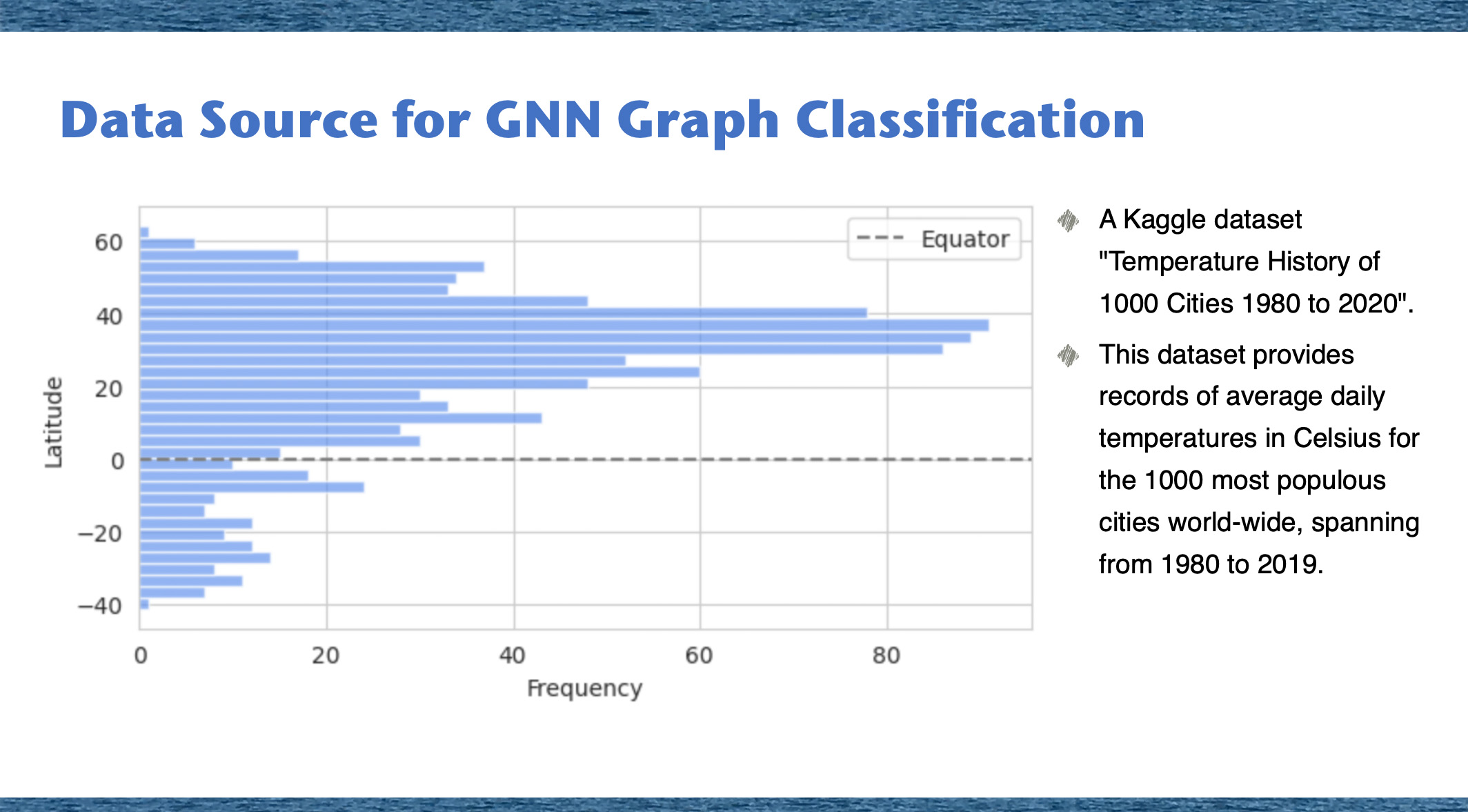
The bar chart shows city frequency by latitude. Most cities are between 20 and 60 degrees in the Northern Hemisphere. There are fewer cities around the equator and even fewer in the Southern Hemisphere.

Sliding Window Graph GNN Graph Classification

Using a 40-year dataset of daily temperatures from 1000 cities, our study evaluates GNN’s effectiveness in identifying global climate patterns. We focus on data from January 1st to the start of each month, providing insights into climate consistency, seasonal changes, and long-term shifts.

Sliding Window Analysis for Global Climate Data.

In our global climate data analysis, we use the sliding window graph method on a dataset with 40 years of daily temperatures from 1000 cities. This approach segments the data into graphs, each defined by a 30-day window (𝑊 = 30) with a 7-day shift (𝑆 = 7), effectively capturing local climate dynamics. This results in 1624 small graphs, allowing us to analyze short-term climate variations and trends.

Our accuracy metrics provide insights into the stability and variability of global climate patterns. High accuracy suggests predictable seasonal trends, while lower accuracy indicates irregular climate patterns or shifts. The sliding window graph method allows us to thoroughly evaluate the model’s ability to identify complex patterns in large climate datasets.

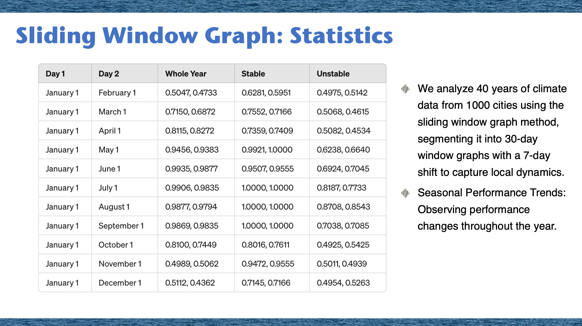
When examining closely spaced months, such as January 1st to February 1st and January 1st to December 1st, the GNN model’s accuracy around 0.5 suggests difficulty in identifying distinct climate patterns. This low accuracy points to potential variability and unpredictability in global weather patterns during these periods, highlighting the complex dynamics of weather.

For periods between January and months like March, April, or October, the model achieves accuracy metrics averaging around 0.7 to 0.8, indicating moderate success in capturing climatic patterns. This is likely due to the model’s proficiency in identifying consistent seasonal transitions over these extended timeframes.

The highest accuracy metrics, ranging from 0.94 to 0.99, are observed for months other than January, such as May, June, July, August, and September. These results reflect the model’s exceptional performance in predicting climate patterns during these months, particularly in the stable summer months. This suggests that the GNN model excels in recognizing and adapting to distinctive climatic patterns, resulting in highly accurate predictions.

Sliding Window Analysis for Stable and Unstable Climate Data.

For classification, we split our graph dataset into ‘stable’ and ‘unstable’ groups based on average cosine similarities between consecutive years. This method segmented the global dataset into stable and unstable categories for our sliding window analysis. Using 20,000 city-year combinations, we set a window size of 30 (𝑊 = 30) and a shift size of 6 (𝑆 = 6), facilitating precise computations for both stable and unstable datasets. Each graph contains 30 nodes (𝐺 = 30), with a shift of 4 (𝑆𝑔 = 4) between successive graphs, resulting in a total of 1648 small graphs.

In our study, GNN graph classification for stable climate cities starts with moderate accuracy in February, significantly improves by May reaching a peak of 100%, and maintains high accuracy through the summer months, only to dip in October with a slight recovery in November. In contrast, unstable climate cities start with near-random accuracy in February, improve steadily, peak in August, and then decline sharply, returning to early-year levels by December. This indicates the model’s varying adaptability to stable and unstable climate patterns throughout the year.

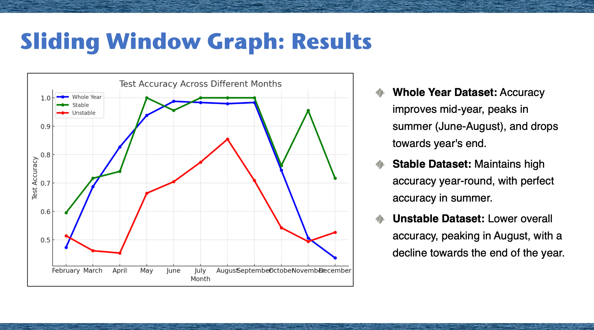
Analysis starting from January 1 shows that the model’s performance is influenced by the time of year. Unstable climates see low accuracies in the early and late parts of the year, suggesting limited learning during these periods. Conversely, stable climates exhibit significant improvements in accuracy during spring and summer, indicating effective data integration. However, the model’s performance overall is subject to fluctuations, peaking in the summer months before declining towards the end of the year, highlighting the challenges in generalizing across seasonal variations in climate data.

Code Details

The create_segments_df function segments a specified column from a DataFrame into fixed-size windows. For each segment, it adds context such as the start date, row index, and column label. The function then combines these segments into a new DataFrame. This is useful for time series analysis or preparing data for machine learning models.

def create_segments_df(df, column_name, window_size, shift,columnLabel):
    segments = []
    for i in range(0, len(df) - window_size + 1, shift):
        segment = df.loc[i:i + window_size - 1, [column_name]].reset_index(drop=True)
        segment = segment.T  # Transpose to get the segment as a row
        segment['start_date'] = df['date'][i]
        segment['rowIndex'] = df['rowIndex'][i]
        segment['theColumn'] = column_name
        segment['columnLabel'] = columnLabel
        segments.append(segment)
    return pd.concat(segments, ignore_index=True)

The group_segments function takes a DataFrame of segments and groups them into larger segments based on specified sizes and shifts. It adds a group index to each group and combines them into a new DataFrame. This is useful for aggregating data over larger windows, essential for graph-based models or detailed data analysis.

def group_segments(segments_df, group_size, group_shift):
    grouped_segments = []
    group_index = 0  
    for i in range(0, len(segments_df) - group_size + 1, group_shift):
        group = segments_df.loc[i:i + group_size - 1].reset_index(drop=True)
        group['graphIndex'] = group_index  # Assign group index
        grouped_segments.append(group)
        group_index += 1  
    return pd.concat(grouped_segments, ignore_index=True)

Take columns col1 and col2 from a dataset, fill NaN values in with their mean values and scale these columns using MinMaxScaler.

from sklearn.preprocessing import MinMaxScaler
scaler = MinMaxScaler()
fx_data=df
if col1 in fx_data.columns:
    fx_data[col1] = fx_data[col1].fillna(fx_data[col1].mean())
    fx_data[col1] = scaler.fit_transform(fx_data[[col1]])
if col2 in fx_data.columns:
    fx_data[col2] = fx_data[col2].fillna(fx_data[col2].mean())
    fx_data[col2] = scaler.fit_transform(fx_data[[col2]])

The code creates segments from two columns (col1 and col2) of a dataset using the create_segments_df function, assigns node indices to each segment, and then groups these segments with the group_segments function. It combines the grouped segments into a final dataset, assigning a unique datasetIdx to each. Finally, it generates metadata for each dataset index and merges it with the segment data to form graphList.

columnLabel=0
segments1 = create_segments_df(df, col1, window_size, shift, columnLabel)
columnLabel=1
segments2 = create_segments_df(df, col2, window_size, shift, columnLabel)
segments1['nodeIndex']=segments1.index
segments2['nodeIndex']=segments2.index
grouped_segments1 = group_segments(segments1, group_size, group_shift)
grouped_segments2 = group_segments(segments2, group_size, group_shift)
dataSet= pd.concat([grouped_segments1, grouped_segments2], ignore_index=True)
dataSet['datasetIdx']=dataSet['columnLabel']*graphMax+dataSet['graphIndex']
dataSubset = dataSet[['datasetIdx','graphIndex','columnLabel','theColumn']].drop_duplicates()
graphMeta = dataSet.groupby([ 'datasetIdx'])['start_date'].agg(['min', 'max'])
graphList = pd.merge(dataSubset, graphMeta, on='datasetIdx')

Continuation of coding is described in our previous study, “GNN Graph Classification for Climate Change Patterns: Graph Neural Network (GNN) Graph Classification - A Novel Method for Analyzing Time Series Data”. This current work continues the same coding methodology for both city graphs and sliding window graphs.

Comparison of GNN Graph Classification Methods.

In this research, we evaluated two distinct GNN Graph Classification techniques for analyzing climate data: the city-graph and the sliding window graph methods. The city-graph method assigns a node to each city-year pair, connecting them based on the cosine similarity of their temperature profiles, making it particularly suited for analyzing long-term climate trends. In contrast, the sliding window technique divides time series data into overlapping segments to form graphs, adeptly identifying short-term climate variations.

Both techniques were applied to the same dataset to compare their effectiveness in categorizing cities by climate stability. We found that the city-graph method more accurately discerned long-term climate stability, whereas the sliding window approach excelled in detecting short-term climate changes. Therefore, the choice of method depends on the specific objectives of the analysis: the city-graph is preferable for examining extended trends, while the sliding window method is ideal for investigating immediate climatic shifts.

In Conclusion

GNN graph classification has shown its strength in mapping complex relationships within graph-based datasets, making it a versatile tool in fields ranging from molecular dynamics to social network analysis. This versatility extends to climate data analysis, where it aids in identifying stable versus unstable climate patterns across cities by evaluating average cosine similarities of yearly temperature fluctuations. The addition of the sliding window graph approach further refines our study, enabling the model to continuously integrate new data and offer a detailed view of changing climate patterns. This technique is adept at capturing the dynamic nature of climate data, allowing for a more nuanced analysis of temporal trends and making it particularly suitable for managing the variable nature of climate data. This method’s ability to prioritize recent data over older information is crucial for adapting to the fast-paced changes characteristic of climate patterns.

In this study, we have leveraged GNN graph classification to address the complex challenge of analyzing climate patterns across different geographic locales, underscoring the method’s adaptability and broad applicability. Our research aimed explicitly at harnessing the potential of GNNs to distinguish between stable and unstable climate conditions in cities worldwide, using average cosine similarities of annual temperature variations as a novel classification metric. By integrating the sliding window graph approach, we have enhanced our model’s ability to dynamically assimilate and refresh data, offering a granular perspective on the fluctuating climate patterns and their implications over time.

This investigation has demonstrated that while equatorial cities exhibit consistency in climate stability, higher latitude cities experience more pronounced fluctuations. Remarkably, our analysis also brought to light certain anomalies, such as Mediterranean cities with unexpectedly consistent climates and cities in China and Mexico with notable climate variability. These findings highlight the critical importance of considering local geographical and climatic factors in climate studies and underscore the nuanced capabilities of GNN models in detecting subtle climate dynamics.

Ultimately, our study reinforces the utility of GNN graph classification, especially with the incorporation of the sliding window approach, as a potent tool for dissecting and understanding climate data. This method does not merely augment the predictive accuracy of our models but significantly bolsters their adaptability to ongoing climate changes, offering a richer comprehension of the complex interplay of factors influencing global climate trends. As such, GNN graph classification emerges as an indispensable instrument in the ongoing efforts to tackle the multifaceted challenges posed by global climate change, paving the way for more informed and effective climate resilience strategies.

• ← Previous Post
• Next Post →