Introduction
Graphs are everywhere in our lives. They represent molecules in chemistry, roads in navigation, and our social networks like Facebook. From molecules to city maps and social network graphs, graphs allow us to model complex relationships in ways that are easy to analyze and visualize.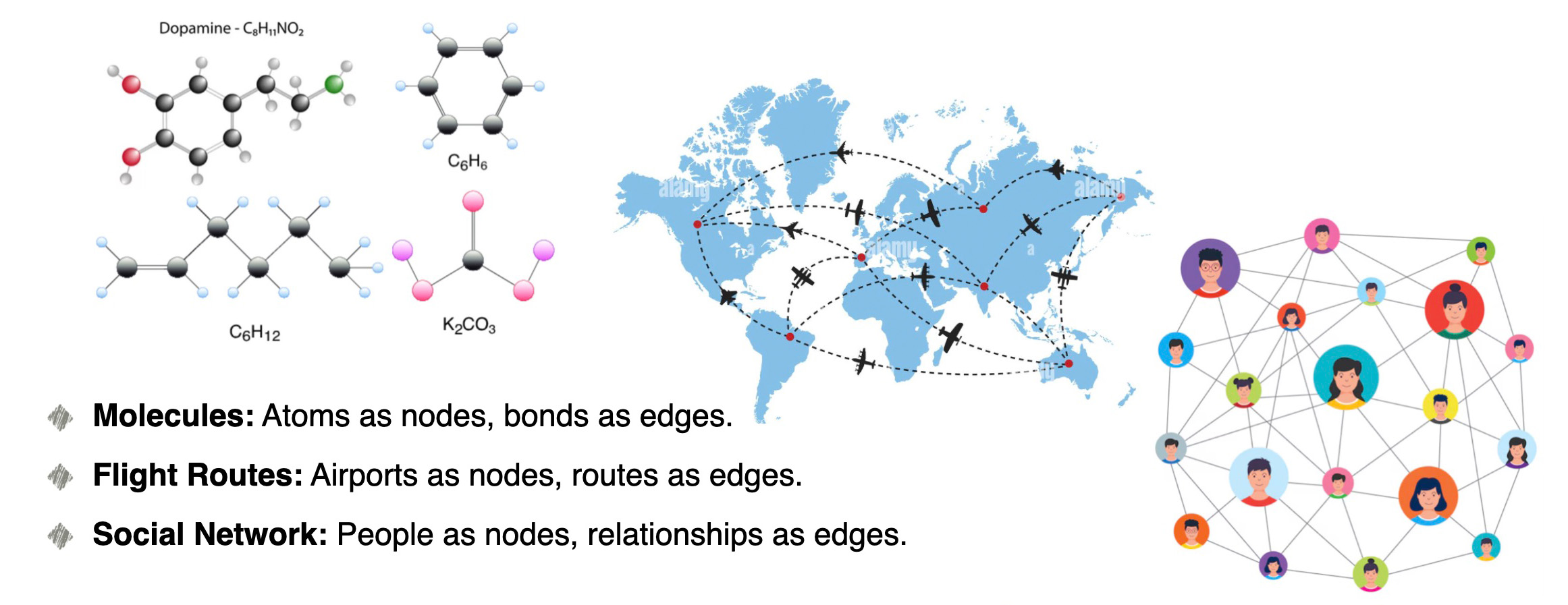 People don’t think sequentially, especially when solving complex problems. Instead, our brains rely on networks of connections, enabling dynamic and non-linear thinking. Graph Neural Networks (GNNs) replicate this process by modeling data as graphs, helping uncover hidden relationships and patterns in everything from neuroscience to social networks.
Building on this, we explore how multi-feature graphs can capture the complexity of real-world systems by representing countries as nodes and their relationships (like borders) as edges. Nodes aren't just static entities—they hold rich features, which might be time series, text, images, or other data that can be represented as vectors. For this study, we focus on time series features, such as life expectancy, GDP, and CO₂ emissions, where each feature may follow a different format.
Using a country geo graph, where edges represent shared borders (land or sea) and nodes represent countries with diverse features, we leverage GNNs for link prediction to embed these features into consistent vector representations. Borders in this graph act as connections that influence cross-country relationships, akin to synapses between neurons. The quality of these connections, such as the openness or type of borders, can provide meaningful insights into the dynamics of international relationships.
This approach allows us to harmonize diverse datasets into a single unified graph, which can then be analyzed for clustering, classification, and prediction tasks. By incorporating details like border types and shared attributes, we aim to better understand how spatial relationships shape global patterns in health, economy, and environment.
Our study highlights the potential of multi-feature graphs in uncovering hidden connections and patterns in global data. By combining spatial relationships, detailed node features, and advanced GNN techniques, we provide a robust framework for analyzing international dynamics and their impact on socio-economic outcomes.
Methods
Pipeline Overview
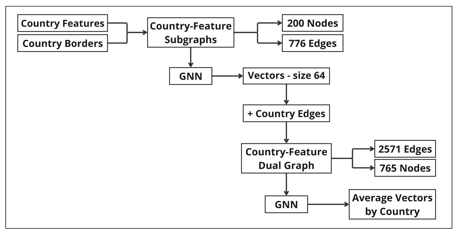
The methodology integrates country features and border information to construct a unified graph, enabling comprehensive analysis of global relationships:
- Country-Feature Subgraphs: Edges are based on land and sea borders, representing geographical connections. Subgraphs were enriched with attributes such as life expectancy, GDP, and internet usage, combining spatial relationships with socio-economic and health data.
- Unified Dual-Layer Graph: Subgraphs were combined into a dual-layer graph by adding intra-country edges that link nodes corresponding to the same country across different features.
- Final Embeddings: A second GNN was applied to the dual-layer graph to generate final embeddings. These embeddings integrate the combined graph structure and relationships across all features and borders.
- Country-Level Aggregation: Node embeddings were aggregated at the country level, creating average vectors that summarize each country’s overall profile, incorporating its socio-economic features and geographic relationships.
- GNN Link Prediction: A Graph Neural Network (GNN) was applied to each subgraph using the GraphSAGE Link Prediction model, embedding time-series features of varying lengths into fixed-size vectors. The Deep Graph Library (DGL) framework was used for efficient training and evaluation, capturing both feature-based and structural relationships.
Graph Construction
We began by constructing a graph where countries were represented as nodes, and edges corresponded to borders between countries. Nodes were identified using country codes, and edges were created for countries sharing either land or sea borders. This foundational graph structure captures geographic connectivity and serves as the basis for modeling socio-economic relationships between countries.
Node Features
Each node (country) was enriched with features derived from publicly available time series datasets, including indicators such as life expectancy, GDP, population, and internet usage rates. These features were preprocessed and normalized to ensure comparability across countries. The inclusion of these diverse node features enabled us to capture multiple aspects of country dynamics and facilitate meaningful graph analysis.
Multiple Feature Sets
To capture the unique influence of each node feature, we constructed separate subgraphs for each feature type. For example, one subgraph was based on life expectancy, while another was based on GDP. Each subgraph retained the same graph structure but focused on a single feature set. We applied GNNs independently to these subgraphs, generating feature-specific embeddings for each country. These embeddings reflected the specific relationships and patterns associated with individual features, such as health, economy, or technology.
GNN Link Prediction
To reveal hidden connections and enrich the graph's structure, we employed GNN Link Prediction as a core component of our methodology. By leveraging the graph’s structure and node features, this approach allowed us to uncover previously unobserved relationships and enhance the graph's utility for analysis.
For this task, we used the GraphSAGE Link Prediction model, implemented via the Deep Graph Library (DGL). GraphSAGE generates robust node embeddings by aggregating information from neighboring nodes and their attributes, with the added advantage of generalizing to unseen nodes without requiring retraining. Our implementation utilized two GraphSAGE layers, progressively refining node representations by combining details from nearby nodes.
The embeddings generated through this process not only captured the individual node features but also the relationships inferred from the graph structure. This methodology facilitated the discovery of hidden connections between countries, which were represented as additional edges in the graph. Similar techniques have been successfully applied to datasets such as the Enron email dataset, demonstrating the effectiveness of GNN-based models in uncovering complex relationships.
Unified Graph Representation
To integrate multiple feature-specific embeddings into a single framework, we constructed a unified graph representation. This involved either aggregating embeddings (e.g., averaging across features) or adding new edges to represent feature-based connections between the same nodes across subgraphs. The unified graph enables a holistic view of country relationships by combining diverse aspects such as health, economy, and connectivity into a single, cohesive structure.
We further propose extending this approach to multi-domain knowledge graphs by linking subgraphs through shared entities. For example, in our study, country nodes are shared across subgraphs representing different domains (e.g., health, economic, and environmental indicators). This linking process enhances the graph's expressiveness and enables the modeling of inter-domain relationships.
Applications and Challenges
The unified graph representation opens up possibilities for various tasks, such as clustering, link prediction, and scenario analysis. By leveraging GNNs, this approach offers flexible and interpretable models for analyzing complex international relationships.
However, constructing knowledge graphs for diverse domains presents challenges, particularly in defining graph structures. For spatial data, graph structures can be based on geographic coordinates. For countries, neighbors are defined by shared borders. Other domains, however, may require unique criteria to establish connections.
By combining embeddings from multiple subgraphs and linking them through shared nodes, we create a scalable framework for multi-domain knowledge graphs. This framework enables comprehensive analyses of interconnected systems and uncovers patterns across diverse datasets, making it a robust tool for addressing complex, real-world challenges.
Experiments
Graph Edges: Data Sources and Data Preparation
Borders between countries can be compared to synapses between neurons, serving as points of connection or division. The nature and quality of these connections evolve over time: open borders foster stronger connections and collaboration between countries, while closed borders often signify increased tension or conflict. This dynamic makes borders a critical factor in understanding international relationships. To define neighboring countries, we rely on information about shared borders. Identifying pairs of countries that share borders is particularly valuable, especially when enriched with data about the type and quality of these borders—such as how easily people or goods can cross them. This additional context provides deeper insights into cross-country interactions and their socio-political implications. There are two primary types of country borders: land borders and sea borders. Each type offers unique insights into the nature of geographic and economic connectivity, making them essential elements in analyzing global relationships.Data Sources for Country Land Borders
For this study, we utilized the Natural Earth Admin 0 - Countries dataset, version 5.0.1 (2023), as the primary source for country boundaries and metadata. This dataset provides comprehensive information about country borders, including land boundaries, and includes associated metadata such as GDP, population, and administrative classifications. The data is publicly available under the CC0 1.0 Public Domain Dedication, ensuring accessibility for research and analysis.
This dataset was instrumental in constructing the graph structure for land borders, where countries are represented as nodes and shared land boundaries as edges. By leveraging this dataset, we ensured the accuracy and reliability of the geographic connectivity in the graph representation.
Reference: Natural Earth. "Admin 0 - Countries." Version 5.0.1, Natural Earth, 2023. https://www.naturalearthdata.com
Land Borders: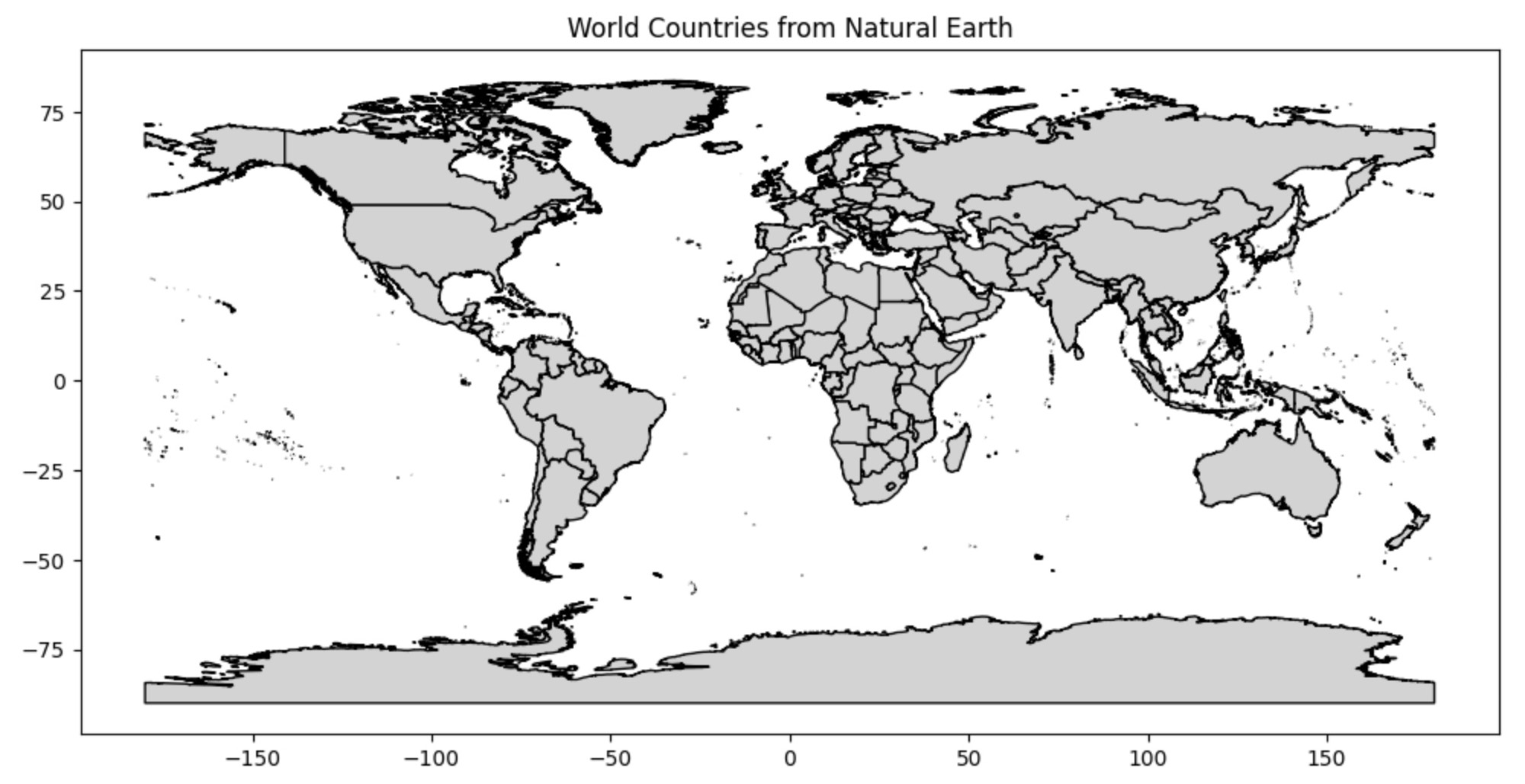
To use datasets stored in Google Drive, we often needed to extract compressed files. Below is an outline of how we unzipped files directly within a Python environment using the zipfile library. This process involved specifying the path to our zip file and the destination directory where the files would be extracted.
Steps we followed:
- Path to the zip file: We located the compressed file in our Google Drive and specified its path.
- Path to extract the files: We chose a destination directory where the contents of the zip file would be extracted.
- Unzip the file: We used Python's zipfile module to extract the contents efficiently.
Below is code for unzipping a file in Google Drive:
import zipfile
import os
zip_file_path = "/content/drive/My Drive/Geo/ne_10m_admin_0_countries.zip"
extract_to_path = "/content/drive/My Drive/Geo/"
with zipfile.ZipFile(zip_file_path, 'r') as zip_ref:
    zip_ref.extractall(extract_to_path)
This approach allows to handle large datasets directly within Google Colab, ensuring seamless integration with your data processing workflow.
Data Source for Country Sea Borders
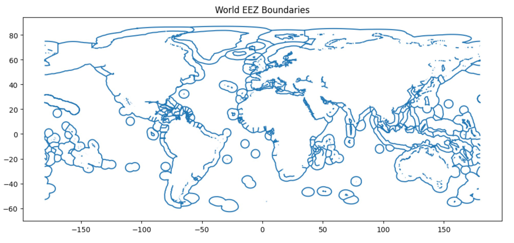
Sea boundaries and Exclusive Economic Zones (EEZs) were obtained from Marineregions.org's World EEZ v12 dataset, version 12 (2023). This dataset provides detailed information on sea boundaries and EEZs and is licensed under the Creative Commons Attribution 4.0 International License (CC BY 4.0). The dataset was used to construct the graph's sea boundaries, where edges represent countries sharing maritime boundaries.
Reference: Marineregions.org. (2023). World EEZ v12 [Dataset]. Version 12. https://www.marineregions.org/.
To work with the World EEZ v12 dataset, we started by locating the ZIP file containing the data. This file was stored in a directory, such as Google Drive, for easy access. Once the file path was identified, a directory was specified for extracting the contents of the ZIP file.
After unzipping the file, the contents of the extracted directory were listed to verify that all necessary files were successfully extracted. This step ensured that the dataset was prepared and ready for further processing and analysis.
import zipfile
import os
zip_file_path = "/content/drive/My Drive/Geo/World_EEZ_v12_20231025_gpkg.zip"
extract_to_path = "/content/drive/My Drive/Geo/World_EEZ_v12_20231025_gpkg/"
with zipfile.ZipFile(zip_file_path, 'r') as zip_ref:
    zip_ref.extractall(extract_to_path)
extracted_files = os.listdir(extract_to_path)
By following these steps, we ensured a seamless workflow for preparing the dataset to incorporate sea boundary data into the graph structure and analysis.
Sea Borders:
Land Neighbors Graph
When integrating multiple datasets with potentially different country naming conventions, it's essential to standardize country names systematically. As part of this process, we used ISO_A3 codes as country indicators instead of country names to ensure consistency across datasets.
To extract land borders as connections (edges) in a graph, we first read the shapefile containing the geographic information. This involves loading the dataset, inspecting its contents, and identifying the relationships between neighboring countries.
For this step, we used the Natural Earth Admin 0 dataset, which provides detailed information about country boundaries. After ensuring the shapefile was loaded correctly, we began processing the data to extract meaningful connections for the graph.
import geopandas as gpd
shapefile_path = "/content/drive/My Drive/natural_earth/ne_110m_admin_0_countries.shp"
world = gpd.read_file(shapefile_path)
Next, we extracted unique country names from the dataset and printed the total number of countries along with their names. This step helped us understand the scope of the dataset and ensured we were working with accurate geographic entities.
To streamline the dataset, we focused on the essential columns required for constructing the graph. These included:
- Country Name: Typically represented by columns like
NAME,SOVEREIGNT, or similar. - Geometry: Contains polygon data defining country borders.
We simplified the dataset by selecting only these columns and renaming the country column for consistency and ease of use in subsequent processing steps. This approach ensured that the dataset remained clean and manageable while retaining all necessary information for building the graph.
world = world[['NAME', 'geometry']]
world = world.rename(columns={'NAME': 'country'})
To identify neighboring countries, we used GeoPandas spatial operations to determine which countries share borders. This step was crucial for defining the edges in our graph, where each edge represents a land border between two countries.
The process involved iterating through each country in the dataset and finding all other countries whose borders touch the geometry of the current country. A dictionary was created to store these relationships, with each country as a key and its list of neighbors as the corresponding value.
To ensure the geometric integrity of the dataset, we first corrected any invalid geometries using a buffer operation, which fixes potential issues with polygon shapes. This step ensured accurate results when performing spatial queries.
world['geometry'] = world['geometry'].buffer(0)
neighbors = {}
for index, country in world.iterrows():
    touching = world[world.geometry.touches(country.geometry)]['country'].tolist()
    neighbors[country['country']] = touching
The resulting dictionary of neighboring countries provided the foundational structure for building the graph’s edges, capturing the geographic connectivity between nodes (countries).
After identifying neighboring countries, the next step was to create the graph representation. Using the dictionary of neighbors, we constructed a graph where nodes represent countries and edges represent shared borders between them.
The process involved initializing an empty graph and iterating through the dictionary. For each country, edges were added to connect it with its neighbors, effectively capturing the geographic relationships between countries.
import networkx as nx
G = nx.Graph()
for country, neighbor_list in neighbors.items():
    for neighbor in neighbor_list:
        G.add_edge(country, neighbor)
This graph structure forms the backbone of our analysis, providing a flexible framework to integrate additional data, such as node features and edge attributes. By visualizing and inspecting the graph, we ensured that the structure accurately reflected the underlying geographic connectivity.
Sea Neighbors Graph
To construct the Sea Neighbors Graph, we first prepared the dataset by extracting the World EEZ v12 files. This dataset provides detailed information about Exclusive Economic Zones (EEZs) and maritime boundaries, making it ideal for identifying sea-based relationships between countries.
The steps included locating the ZIP file containing the dataset, specifying the directory for extraction, and unzipping the file. Once the files were extracted, the directory was inspected to ensure that all necessary components were available for further processing.
import zipfile
import os
zip_file_path = "/content/drive/My Drive/Geo/World_EEZ_v12_20231025_gpkg.zip"
extract_to_path = "/content/drive/My Drive/Geo/World_EEZ_v12_20231025_gpkg/"
with zipfile.ZipFile(zip_file_path, 'r') as zip_ref:
    zip_ref.extractall(extract_to_path)
extracted_files = os.listdir(extract_to_path)
These steps ensured that the dataset was ready for use in building the Sea Neighbors Graph, where edges represent shared maritime boundaries between countries.
When working with geographic data, it is essential to ensure that all geometries are valid to avoid issues during spatial operations. Invalid geometries, such as self-intersecting polygons, can lead to errors or inaccurate results when analyzing spatial relationships.
To address this, we corrected any invalid geometries in the dataset by applying a buffer operation with a distance of zero. This operation is a common technique for fixing minor geometric inconsistencies without altering the overall shape of the polygons.
eez['geometry'] = eez['geometry'].buffer(0)After applying the buffer operation, we confirmed the validity of the geometries. Ensuring valid geometries was a crucial step in preparing the data for constructing the Sea Neighbors Graph and performing reliable spatial queries.
To identify sea neighbors, we analyzed overlapping Exclusive Economic Zones (EEZs) using spatial operations. This process determined which countries share maritime boundaries based on their EEZ polygons.
The method involved iterating through each EEZ polygon in the dataset and checking for intersections with other polygons. For every overlap, we recorded pairs of countries sharing the boundary, ensuring that duplicate pairs were avoided by sorting and storing them uniquely.
This approach allowed us to construct a comprehensive list of sea neighbors, which served as the foundation for creating the Sea Neighbors Graph. Each pair in this list represents a connection (edge) between countries based on their shared maritime boundaries.
country_pairs = []
for index, country in eez_sea.iterrows():
    overlapping_countries = eez_sea[eez_sea.geometry.intersects(country.geometry)]['country'].tolist()
    overlapping_countries = [c for c in overlapping_countries if c != country['country']]
    for neighbor in overlapping_countries:
        pair = tuple(sorted([country['country'], neighbor]))
        if pair not in country_pairs:
            country_pairs.append(pair)
To construct the Sea Neighbors Graph, we converted the list of overlapping EEZ country pairs into a graph structure using NetworkX. Each country was represented as a node, and shared maritime boundaries were represented as edges between the nodes.
The process began by initializing an empty graph and iterating through the list of country pairs. For each pair, an edge was added to the graph, capturing the maritime connection between the two countries. To ensure a clean graph structure, isolated nodes—countries without any maritime neighbors—were identified and removed from the graph.
import networkx as nx
import matplotlib.pyplot as plt
sea_graph = nx.Graph()
for pair in country_pairs:
    sea_graph.add_edge(pair[0], pair[1])
isolated_nodes = list(nx.isolates(sea_graph))
sea_graph.remove_nodes_from(isolated_nodes)
This graph representation forms the basis for analyzing sea-based relationships between countries, enabling visualization and further exploration of maritime connectivity. By incorporating only connected nodes, we ensured that the graph was well-suited for downstream tasks such as clustering, classification, and link prediction.
Combine Land and Sea Graphs
To create a unified representation of geographic relationships, we combined the Land Neighbors Graph and the Sea Neighbors Graph. This unified graph includes all connections based on both land and sea borders, enabling a holistic analysis of country relationships.
The process began by annotating edges in each graph with attributes that indicate the type of connection. For the Land Neighbors Graph, all edges were marked with the attribute 'type': 'land'. Similarly, for the Sea Neighbors Graph, all edges were labeled with 'type': 'sea'.
for u, v in land_graph.edges:
    land_graph[u][v]['type'] = 'land'
for u, v in sea_graph.edges:
sea_graph[u][v]['type'] = 'sea'
Next, the two graphs were combined using NetworkX's composition operation. If an edge existed in both the land and sea graphs, it was marked as 'type': 'both' to indicate that the connection represents both land and sea borders.
combined_graph = nx.compose(land_graph, sea_graph)
for u, v in combined_graph.edges:
    if land_graph.has_edge(u, v) and sea_graph.has_edge(u, v):
        combined_graph[u][v]['type'] = 'both'  # Mark as both land and sea
The resulting combined graph captures the complexity of geographic relationships by integrating both land and maritime connectivity into a single structure. Each node in the graph corresponds to a country, labeled with its ISO 3166-1 alpha-3 code for easy identification. This unified graph serves as a foundation for analyzing various aspects of international relationships and their influence on socio-economic and environmental factors.
This image represents the combined graph of countries connected by both land and sea borders. Each node in the graph corresponds to a country, labeled with its ISO 3166-1 alpha-3 code for easy identification.import matplotlib.pyplot as plt
plt.figure(figsize=(15, 8))
nx.draw(Gedges, with_labels=True, node_size=11,node_color='lightgrey', font_size=9)
plt.show()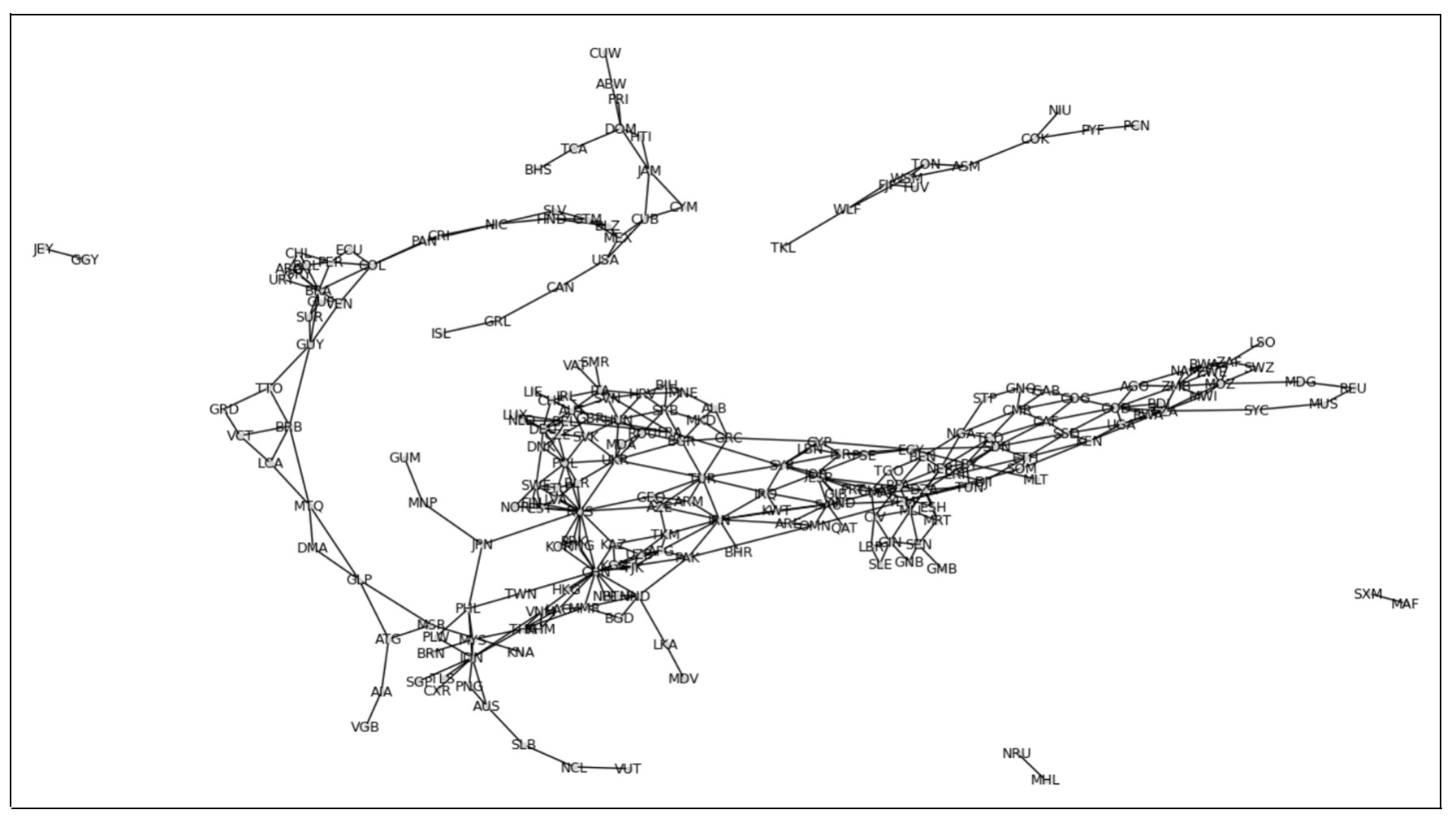
Graph Nodes: Data Sources and Preparation
We constructed graph nodes by incorporating socio-economic and health data from the World Bank:
- Life Expectancy: Extracted from the World Development Indicators (WDI) dataset, capturing the average years a newborn is expected to live.
- Poverty Levels: Percentage of the population living below $2.15 a day (2017 PPP), reflecting economic disparities.
- GDP Per Capita: Measuring economic performance and living standards.
- Internet Usage: Percentage of individuals using the Internet, indicating global connectivity.
World Bank Data Sources for Graph Nodes
The life expectancy dataset was used to create node features in our graph, representing time-series data for each country. This data was cleaned, normalized, and integrated into the graph structure, providing meaningful inputs for predictive modeling and analysis. The life expectancy data was sourced from the World Bank's World Development Indicators (WDI). This dataset provides annual life expectancy figures for countries worldwide, representing the average number of years a newborn is expected to live under current mortality conditions. More information and access to the dataset are available on the World Bank: Life Expectancy. The dataset "Poverty headcount ratio at $2.15 a day (2017 PPP) (% of population)" is sourced from the World Bank's World Development Indicators. It provides data on the percentage of the population living below the international poverty line of $2.15 per day (adjusted for 2017 purchasing power parity). This dataset is publicly available and offers insights into global poverty trends. More information and access to the dataset are available on the World Bank: Poverty. The dataset "GDP per capita (current US$)" is sourced from the World Bank's World Development Indicators. It provides data on the gross domestic product divided by the midyear population, expressed in current U.S. dollars. This dataset is a key indicator for analyzing economic performance and living standards across countries. More information and access to the dataset are available on the World Bank: GDP per capita. The dataset "Individuals using the Internet (% of population)" is sourced from the World Bank Open Data platform. It provides the percentage of individuals in a country who use the Internet and is a valuable resource for analyzing global digital connectivity trends. More information and access to the dataset are available on the World Bank: Individuals using the Internet.Data Process for Country Life Expectancy
The life expectancy data, sourced from the World Bank's World Development Indicators (WDI), provides life expectancy at birth for countries worldwide across multiple years. This publicly accessible dataset is widely used for analyzing health trends and socio-economic development.
The first step was loading and inspecting the dataset to identify relevant columns for analysis. We then filtered and reshaped the data into a usable format for graph-based modeling by:
- Keeping relevant columns, such as country name, country code, and life expectancy values.
- Reshaping the dataset into a long format, with years as variables, for easier integration into the graph structure.
The loading process included skipping the first 4 rows (containing metadata), using a comma as the delimiter, and employing the Python engine for parsing flexibility. These preprocessing steps ensured the dataset was clean, structured, and ready for integration into the graph model.
import pandas as pd
file_path ='/content/drive/My Drive/Geo/API_SP.DYN.LE00.IN_DS2_en_csv_v2_99.csv'
data= pd.read_csv(
    file_path,
    skiprows=4,
    delimiter=",",
    engine="python"
)
For our study, we manually preprocessed life expectancy data to ensure compatibility with the graph structure. This preprocessing was essential for aligning country-level data with the nodes in the graph and maintaining data integrity.
We handled missing values by filling them with zeros, ensuring a complete dataset for integration. Next, we aligned the country codes between the dataset and the graph nodes. This involved extracting nodes from the graph and standardizing country codes to remove inconsistencies.
import pandas as pd
import numpy as np
file_path ='/content/drive/My Drive/Geo/WorldBank/Life_expectancy.csv'
data=pd.read_csv(file_path)
data = data.fillna(0.0)
Then we performed an inner join on the 'Country Code' column to merge the graph nodes with the life expectancy data. This step connected node features to the graph structure, allowing for meaningful analysis and modeling in subsequent stages.
nodes_df = pd.DataFrame(Gedges.nodes, columns=['Country Code'])
nodes_df['Country Code'] = nodes_df['Country Code'].str.strip()
data['Country Code'] = data['Country Code'].str.strip()
merged_data = nodes_df.merge(data, on='Country Code', how='inner')
In our data preprocessing, we addressed the issue of missing values represented as zeros in the dataset. To ensure continuity in the time series data, we replaced all 0.0 values in a row with the closest non-zero value in the same row.
The process involved checking each row for non-zero values. For rows with zeros, we filled these values by propagating the nearest valid data point forward and backward along the row. If an entire row consisted of zeros, it remained unchanged. This approach ensured that gaps in the data were minimized without introducing biases or arbitrary values.
import numpy as np
def replace_zeros_with_closest_nonzero(row):
    non_zero_indices = np.where(row > 0.0)[0]
    if len(non_zero_indices) == 0:
        return row
    for i in range(1, len(row)):
        if row[i] == 0.0:
            row[i] = row[i - 1] if row[i - 1] > 0.0 else 0.0
    for i in range(len(row) - 2, -1, -1):
        if row[i] == 0.0:
            row[i] = row[i + 1] if row[i + 1] > 0.0 else 0.0
    return row
columns_to_process = merged_data.select_dtypes(include=[np.number]).columns
merged_data[columns_to_process] = merged_data[columns_to_process]
  .apply(replace_zeros_with_closest_nonzero, axis=1)
This step was applied to all numerical columns in the dataset, resulting in a cleaned and more consistent dataset that could be effectively used for graph-based analysis and modeling.
After handling missing values, we proceeded to clean the dataset further by dropping rows containing NaN values. This step ensured that the dataset was fully prepared for graph-based analysis, free of incomplete data entries.
Next, we reshaped and normalized the data to enhance its comparability and suitability for cosine similarity computations. The time series data, excluding identifiers like country codes and names, underwent L2 normalization. This technique scales each row to have a unit norm, emphasizing relative patterns over absolute magnitudes.
import numpy as np
from sklearn.preprocessing import normalize
time_series_data = merged_data.iloc[:, 2:].values
normalized_data = normalize(time_series_data, norm='l2', axis=1)
merged_data.iloc[:, 2:] = normalized_data
By replacing the original columns with the normalized data, we created a consistent dataset optimized for similarity calculations and embedding processes in the graph model.
After preprocessing the dataset, we filtered the graph nodes to include only those with corresponding time series data. This step ensured that the graph structure and the dataset were fully aligned for analysis.
We identified valid nodes by matching country codes in the graph with those in the processed dataset. Using this information, a subgraph was created from the original graph, retaining only the nodes with associated time series data.
For each valid node in the filtered graph, we added its corresponding time series data as a node attribute. This enriched the graph structure, embedding meaningful data into the nodes for downstream tasks such as clustering, classification, and link prediction.
valid_nodes = set(merged_data['Country Code'])
filtered_graph = Gedges.subgraph(valid_nodes).copy()
for node in filtered_graph.nodes:
    node_data = merged_data.loc[merged_data['Country Code'] == node].iloc[:, 2:].values
    filtered_graph.nodes[node]['time_series'] = node_data[0]
To integrate node features effectively into the graph, we first extracted country codes and created a mapping table linking node identifiers to their respective country codes. This process ensures that each node in the graph is associated with its corresponding country.
The steps involved include:
- Extracting country codes from the graph nodes. This step checks whether the node contains a 'Country Code' attribute, ensuring accurate alignment between the graph and the dataset.
- Preparing a mapping table that connects each node ID to its country code. This mapping serves as a crucial link between the graph structure and external data.
- Adding a 'Feature' column to the mapping table. In this case, we associated the literal value "Life expectancy" to signify the feature type being analyzed for the nodes.
This mapping table not only links the graph structure to external data sources but also helps streamline the integration of additional node features for future analysis.
import pandas as pd
import networkx as nx
country_code_mapping = {
    node: filtered_graph.nodes[node]['Country Code']
    if 'Country Code' in filtered_graph.nodes[node]
    else node for node in filtered_graph.nodes
}
mapping_table = pd.DataFrame({
    'Node ID': list(country_code_mapping.keys()),
    'Country Code': list(country_code_mapping.values())
})
mapping_table['Feature'] = "Life expectancy"
mapping_table=mapping_table.reset_index(drop=True)
mapping_table['countryIndex'] = mapping_table.index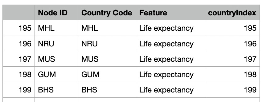
The prepared mapping table was saved as a CSV file for future reference and analysis. This ensures that the relationship between nodes, country codes, and their associated features is preserved and can be reused in subsequent steps.
Saving the mapping table provides a convenient way to link graph nodes to external datasets, enabling seamless integration of node features into the graph structure.
filePath="/content/drive/My Drive/GEO/"
mapping_table.to_csv(filePath+'Life_expectancy_node_mapping.csv', index=False)
Prepare Input Data and Train GNN Link Prediction Model
The model training phase involves preparing the input graph with enriched node features and converting it into a suitable format for processing with Graph Neural Networks (GNNs). The steps include ensuring that the graph nodes are equipped with meaningful attributes, such as time series data, and converting the graph into the Deep Graph Library (DGL) format.
For this study, we assigned the processed time series data as the 'feat' attribute for each node in the filtered graph. This feature represents the life expectancy values or other relevant node features. Each node's feature was converted into a tensor to make it compatible with GNN frameworks.
The enriched NetworkX graph was then converted into a DGL graph using the `from_networkx` method. This step preserved the graph structure and node attributes, ensuring the data was ready for GNN training. The resulting DGL graph structure included 200 nodes, 776 edges, and a feature vector of size 63 for each node, making it suitable for tasks such as link prediction.
import dgl
import torch
import networkx as nx
for node in filtered_graph.nodes:
    time_series = filtered_graph.nodes[node].get('time_series', [])
    filtered_graph.nodes[node]['feat'] = torch.tensor(time_series, dtype=torch.float32)
dgl_graph_nodes = dgl.from_networkx(filtered_graph, node_attrs=['feat'])
g=dgl_graph_nodes
g
Graph(num_nodes=200, num_edges=776,
      ndata_schemes={'feat': Scheme(shape=(63,), dtype=torch.float32)}
      edata_schemes={})
The model training phase leveraged code templates from the Deep Graph Library (DGL). These templates streamlined the process of preparing datasets and implementing the Graph Neural Network (GNN) architecture.
The use of DGL's resources ensured a consistent and efficient approach to building and training the model on our multi-feature country graph.
u, v = g.edges()
eids = np.arange(g.number_of_edges())
eids = np.random.permutation(eids)
test_size = int(len(eids) * 0.1)
train_size = g.number_of_edges() - test_size
test_pos_u, test_pos_v = u[eids[:test_size]], v[eids[:test_size]]
train_pos_u, train_pos_v = u[eids[test_size:]], v[eids[test_size:]]

adj = sp.coo_matrix((np.ones(len(u)), (u.numpy(), v.numpy())))
adj_neg = 1 - adj.todense() - np.eye(g.number_of_nodes())
neg_u, neg_v = np.where(adj_neg != 0)

neg_eids = np.random.choice(len(neg_u), g.number_of_edges())
test_neg_u, test_neg_v = neg_u[neg_eids[:test_size]], neg_v[neg_eids[:test_size]]
train_neg_u, train_neg_v = neg_u[neg_eids[test_size:]], neg_v[neg_eids[test_size:]]
train_g = dgl.remove_edges(g, eids[:test_size])
from dgl.nn import SAGEConv

class GraphSAGE(nn.Module):
    def __init__(self, in_feats, h_feats):
        super(GraphSAGE, self).__init__()
        self.conv1 = SAGEConv(in_feats, h_feats, 'mean')
        self.conv2 = SAGEConv(h_feats, h_feats, 'mean')

    def forward(self, g, in_feat):
        h = self.conv1(g, in_feat)
        h = F.relu(h)
        h = self.conv2(g, h)
        return h
train_pos_g = dgl.graph((train_pos_u, train_pos_v), num_nodes=g.number_of_nodes())
train_neg_g = dgl.graph((train_neg_u, train_neg_v), num_nodes=g.number_of_nodes())
test_pos_g = dgl.graph((test_pos_u, test_pos_v), num_nodes=g.number_of_nodes())
test_neg_g = dgl.graph((test_neg_u, test_neg_v), num_nodes=g.number_of_nodes())

import dgl.function as fn
class DotPredictor(nn.Module):
    def forward(self, g, h):
        with g.local_scope():
            g.ndata['h'] = h
            g.apply_edges(fn.u_dot_v('h', 'h', 'score'))
            return g.edata['score'][:, 0]

class MLPPredictor(nn.Module):
def __init__(self, h_feats):
        super().__init__()
        self.W1 = nn.Linear(h_feats * 2, h_feats)
        self.W2 = nn.Linear(h_feats, 1)

def apply_edges(self, edges):
      h = torch.cat([edges.src['h'], edges.dst['h']], 1)
      return {'score': self.W2(F.relu(self.W1(h))).squeeze(1)}

def forward(self, g, h):
  with g.local_scope():
    g.ndata['h'] = h
    g.apply_edges(self.apply_edges)
    return g.edata['score']
    model = GraphSAGE(train_g.ndata['feat'].shape[1], 64)
    pred = DotPredictor()

def compute_loss(pos_score, neg_score):
    scores = torch.cat([pos_score, neg_score])
    labels = torch.cat([torch.ones(pos_score.shape[0]),
      torch.zeros(neg_score.shape[0])])
    return F.binary_cross_entropy_with_logits(scores, labels)

def compute_auc(pos_score, neg_score):
    scores = torch.cat([pos_score, neg_score]).numpy()
    abels = torch.cat(
        [torch.ones(pos_score.shape[0]),
            torch.zeros(neg_score.shape[0])]).numpy()
    return roc_auc_score(labels, scores)
optimizer = torch.optim.Adam(itertools.chain(model.parameters(),
    pred.parameters()), lr=1e-4 )
The training process iteratively refined the model's parameters through a series of epochs. During each epoch, the model computed embeddings for nodes, predicted scores for positive and negative edges, and calculated the loss function based on these predictions.
An optimizer was employed to minimize the loss by adjusting model parameters through backpropagation. Progress was monitored by printing the loss at regular intervals, providing insight into the model's convergence over time.
all_logits = []
for e in range(4000):
    h = model(train_g, train_g.ndata['feat'])
    pos_score = pred(train_pos_g, h)
    neg_score = pred(train_neg_g, h)
    loss = compute_loss(pos_score, neg_score)
    optimizer.zero_grad()
    loss.backward()
    optimizer.step()
    if e % 100 == 0:
        print('In epoch {}, loss: {}'.format(e, loss))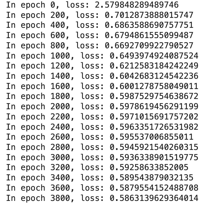
To evaluate the model's performance, we computed the Area Under the Receiver Operating Characteristic Curve (AUC) score. Using the predictions for positive and negative edges on the test dataset, the AUC score measures the model's ability to distinguish between actual connections and non-connections in the graph.
In this case, the model achieved an AUC of 0.787, indicating a strong predictive capability for link prediction tasks within the country graph.
from sklearn.metrics import roc_auc_score
with torch.no_grad():
    pos_score = pred(test_pos_g, h)
    neg_score = pred(test_neg_g, h)
    print('AUC', compute_auc(pos_score, neg_score))
AUC 0.7874852420306966
Getting Embedding Vectors from GNN Link Prediction Model
To extract and save the learned embedding vectors from the trained Graph Neural Network (GNN) Link Prediction model, we followed these steps:
First, the embeddings, stored as a PyTorch tensor (`h`), were converted to a NumPy array for easier handling. The resulting embedding table was structured as a DataFrame, with each row representing the embedding vector for a corresponding node.
An additional column, `countryIndex`, was added to the embedding table, linking each vector to its respective node identifier. This table was then merged with the previously created mapping table, which contains country codes and node details, ensuring that each embedding vector was correctly associated with its corresponding country.
The final table, containing country codes and their respective embedding vectors, was saved as a CSV file for further analysis and integration into downstream tasks.
import pandas as pd
import torch
h_numpy = h.detach().numpy()
embedding_table = pd.DataFrame(h_numpy)
embedding_table['countryIndex'] = embedding_table.index
final_table = mapping_table.merge(embedding_table, on='countryIndex', how='inner')
final_table.to_csv(filePath+'Life_expectancy_embeddings.csv', index=False)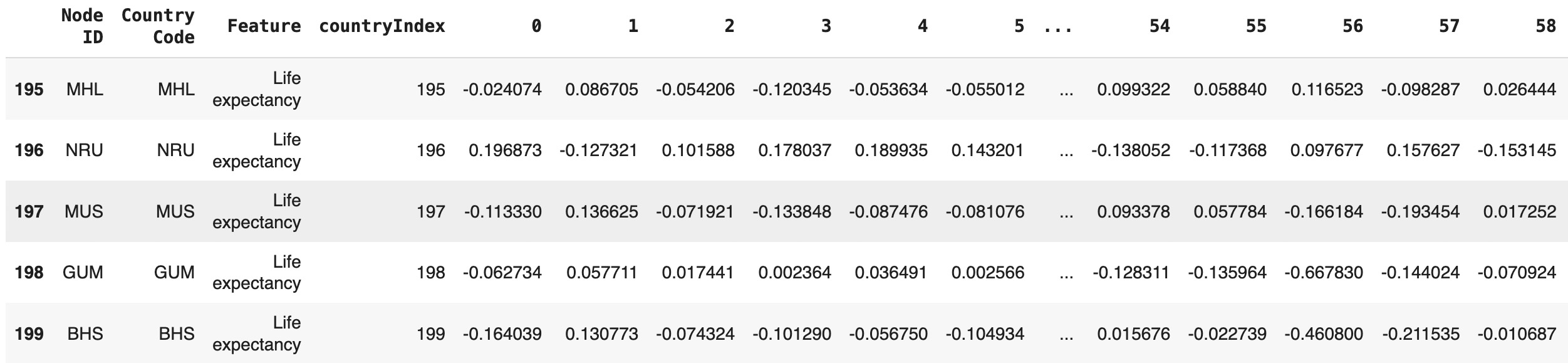
Unified Graph of Subgraphs
To create a unified graph that integrates multiple subgraphs based on different features, we started by combining node data from various datasets. Each dataset represents a specific feature, such as life expectancy, GDP per capita, or poverty levels. These datasets were merged to establish a common structure for the graph.
We concatenated the feature-specific data files into a single DataFrame, ensuring that all relevant attributes were retained. To uniquely identify each node, we created a composite identifier by combining the country code and feature type into a new column, country_feature. This ensures that nodes from different features are distinctly represented, even if they share the same country code.
Additionally, a globalIndex column was introduced, assigning a unique index to every node in the combined dataset. This index simplifies the process of creating edges and constructing the unified graph.
data1 = pd.read_csv(filePath+'Life_expectancy_embeddings.csv')
data2 = pd.read_csv(filePath+'GDP_per_capita_embeddings.csv')
data3 = pd.read_csv(filePath+'Poor_embeddings.csv')
data4 = pd.read_csv(filePath+'Internet_embeddings.csv')
dataNodes = pd.concat([data1, data2, data3, data4], ignore_index=True)
dataNodes['country_feature'] = dataNodes['Country Code'] + "~" + dataNodes['Feature']
dataNodes['globalIndex'] = dataNodes.indexTo integrate the edges of different subgraphs into a unified graph, we processed the relationships for each feature independently. By iterating over the feature-specific data, we linked the nodes within the graph structure based on their corresponding edges.
For each feature (e.g., "Poor", "GDP per capita", "Internet", and "Life expectancy"), the following steps were performed:
- Filtered the combined node dataset to isolate nodes associated with the current feature.
-
Created a mapping from country codes to their respective
globalIndex. -
Iterated through the edges of the initial graph (
Gedges) and identified valid connections where both nodes were present in the current feature dataset. - Stored the identified edges for each feature in a separate list.
This approach ensured that the relationships specific to each feature were preserved while preparing for the construction of the unified graph. The resulting lists of edges will be used to represent the connections within the multi-feature graph model.
features = ['Poor', 'GDP per capita','Life expectancy','Internet']
edges_for_global = []
for feature in features:
    filtered_data = dataNodes[dataNodes['Feature'] == feature]
    country_to_index =
      filtered_data.set_index('Country Code')['globalIndex'].to_dict()
    edges_for_feature = []
    for edge in Gedges.edges:
        left, right = edge
        left_index = country_to_index.get(left)
        right_index = country_to_index.get(right)
        if left_index is not None and right_index is not None:
            edges_for_feature.append((left_index, right_index))
    edges_for_global.append(edges_for_feature)
To further enrich the unified graph, we established edges between nodes that shared the same country code. This step aimed to capture intrinsic relationships between features within the same country.
The process involved:
-
Grouping
globalIndexvalues by country codes using the combined dataset (dataNodes). -
Iterating through each group of
globalIndexvalues and adding edges between all possible pairs of indices within the same group.
The generated edges capture the multi-feature connections for each country, enhancing the unified graph's structure. These new edges were combined with the previously identified feature-specific edges to form a comprehensive representation of the graph.
global_index_mapping = dataNodes.groupby('Country Code')['globalIndex']
  .apply(list).to_dict()
edges_with_equal_country_codes = []
for country_code, global_indices in global_index_mapping.items():
    for i in range(len(global_indices)):
        for j in range(i + 1, len(global_indices)):
edges_for_global.append(edges_with_equal_country_codes)
To finalize the unified graph, we flattened the list of edges derived from feature-specific and country code-based connections. This step ensures that all edges are combined into a single, cohesive structure.
The process involved:
-
Flattening
edges_for_global, which contains edges grouped by features, into a single list of edges. -
Initializing a new graph and adding all edges to it using the
add_edges_frommethod from NetworkX.
The resulting unified graph incorporates both inter-feature relationships and intra-country connections, providing a robust framework for further analysis.
import networkx as nx
all_edges = [edge for feature_edges in edges_for_global for edge in feature_edges]
new_graph = nx.Graph()
new_graph.add_edges_from(all_edges)GNN Link Prediction and Cross-Country Analysis
In our study, we created a unified graph that combines multiple perspectives of country relationships. Each node in the graph represents a unique combination of a country and one of its features, such as life expectancy, GDP per capita, or poverty levels. Edges in the graph capture two types of connections: shared borders between countries and relationships where features belong to the same country. This dual-layer graph structure allows us to explore both geographical and intra-country relationships simultaneously, offering a comprehensive view of global dynamics.
The next phase involves leveraging this unified graph for deeper insights. Using a Graph Neural Network (GNN) Link Prediction model, we aim to uncover hidden connections and patterns within the graph. The GNN will generate embedded vectors for each node, capturing both the node's individual features and its position in the graph structure.
Once the embeddings are generated, we will aggregate the vectors at the country level. This step ensures that the diverse feature representations for each country are unified into a single vector, encapsulating the country's overall profile. By applying linear algebra techniques to these aggregated vectors, we will measure similarities between countries, enabling a data-driven comparison of global trends in health, economy, and connectivity.
This approach highlights the potential of GNNs in analyzing multi-faceted relationships and provides a robust framework for comparing countries based on diverse and complex data. It is a step forward in understanding global patterns and uncovering insights from interconnected datasets.
Using the dgl.from_networkx method, the NetworkX graph was converted to the DGL format. This transformation preserved the graph structure and enriched each node with a 64-dimensional feature vector, preparing the graph for GNN-based link prediction and analysis tasks.
nodes_with_edges = set(index for feature_edges
    in edges_for_global for edge in feature_edges for index in edge)
filtered_dataNodes = dataNodes[dataNodes['globalIndex'].isin(nodes_with_edges)]
dgl_graph = nx.Graph()
all_edges = [edge for feature_edges in edges_for_global for edge in feature_edges]
dgl_graph.add_edges_from(all_edges)
node_features = filtered_dataNodes.iloc[:, 4:-2].apply(pd.to_numeric, errors='coerce')
node_features = node_features.fillna(0).values
new_graph_dgl = dgl.from_networkx(dgl_graph)
new_graph_dgl.ndata['features'] = torch.tensor(node_features, dtype=torch.float32)
new_graph_dgl
Graph(num_nodes=765, num_edges=5142,
      ndata_schemes={'features': Scheme(shape=(64,), dtype=torch.float32)}
      edata_schemes={})
The GNN Link Prediction model was trained as described earlier, achieving an impressive AUC score of 0.8720. This result highlights the model's strong capability to predict connections within the unified graph, reflecting the underlying relationships between country-feature pairs.
Using the trained model, positive and negative edge scores were evaluated on the test set. The Area Under the Receiver Operating Characteristic Curve (AUC) was calculated, providing a robust measure of the model's performance.
from sklearn.metrics import roc_auc_score
with torch.no_grad():
    pos_score = pred(test_pos_g, h)
    neg_score = pred(test_neg_g, h)
    print('AUC', compute_auc(pos_score, neg_score))
AUC 0.8720230434980092import pandas as pd
import torch
h_numpy = h.detach().numpy()
h_df = pd.DataFrame(h_numpy)
h_df['globalIndex'] = h_df.index
nodes=nodes[['Country Code', 'Feature','globalIndex']]
h_nodes = pd.merge(nodes, h_df, on='globalIndex', how='inner')Aggregating Node Embeddings by Country
To analyze the data at the country level, we calculated the average embedding vectors for eachCountry Code. This process involved grouping the unified table (h_nodes) by Country Code, computing the mean for all embedding columns, and resetting the index to ensure Country Code remained a visible column. The resulting average_vectors table provides a single, unified vector for each country, capturing multidimensional relationships across features.
embedding_columns = h_nodes.columns[3:]
average_vectors = h_nodes.groupby('Country Code')[embedding_columns].mean()
average_vectors = average_vectors.reset_index()
To make the dataset more interpretable, we enriched the average_vectors table by mapping each Country Code to its corresponding Country Name. This was accomplished using the pycountry library, which provides reliable mappings between ISO 3166-1 alpha-3 country codes and their official country names. The resulting table now includes country names alongside the country codes and embedding vectors, enhancing clarity and usability for further analysis.
import pandas as pd
import pycountry
def get_country_name(iso_code):
    try:
        country = pycountry.countries.get(alpha_3=iso_code)
        return country.name if country else None
    except Exception:
        return None
average_vectors['Country Name'] = average_vectors['Country Code'].apply(get_country_name)
Interpreting Model Results: Cosine Similarity
Using node embeddings, we calculated cosine similarities to explore relationships between countries. This method captures similarities across various dimensions, such as health, economy, and connectivity. Cosine similarity analysis serves as a basis for comparative studies, helping to identify shared challenges or opportunities and informing policy-making decisions.
import pandas as pd
from sklearn.metrics.pairwise import cosine_similarity
from itertools import combinations
vectors = average_vectors.iloc[:, 1:-1].values
countries_info = average_vectors[['Country Code', 'Country Name']]
results = []
for (idx1, row1), (idx2, row2) in combinations(countries_info.iterrows(), 2):
    cos_sim = cosine_similarity([vectors[idx1]], [vectors[idx2]])[0][0]
    results.append({
        'Country Code 1': row1['Country Code'],
        'Country Code 2': row2['Country Code'],
        'Country Name 1': row1['Country Name'],
        'Country Name 2': row2['Country Name'],
        'Cosine Similarity': cos_sim
    })
cosine_similarity_df = pd.DataFrame(results)def get_border_type(graph, source, target):
if graph.has_edge(source, target):
return graph[source][target].get('type', 'unknown')
else:
return 'no border'
cosine_similarity_df['Border Type'] = cosine_similarity_df.apply(
lambda row:
get_border_type(Gedges, row['Country Code 1'], row['Country Code 2']), axis=1
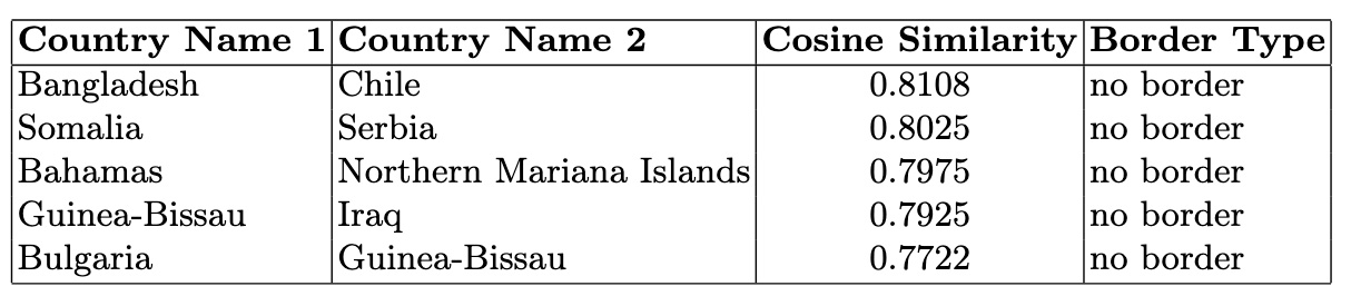
)High Similarity Countries Without Borders: This analysis identifies country pairs with high cosine similarity (> 0.78) but no shared borders. These pairs reveal strong feature-based relationships, such as economic or health similarities, independent of geographical proximity. Such insights highlight potential partnerships or shared challenges among geographically distant nations.
high_similarity_no_border = cosine_similarity_df[
    (cosine_similarity_df['Cosine Similarity'] > 0.77)
       & (cosine_similarity_df['Border Type'] == 'no border')
]
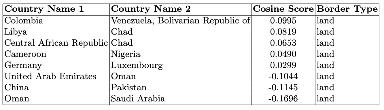
Low Similarity Countries With Borders: This analysis explores neighboring countries with low cosine similarity (e.g., <0.1). These pairs highlight geographical neighbors that exhibit distinct socio-economic or cultural differences, offering insights into contrasts despite shared borders.
low_similarity_with_border = cosine_similarity_df[
    (cosine_similarity_df['Cosine Similarity'] < 0.1)
    & (cosine_similarity_df['Border Type'] == 'land')
]
To identify the most similar country pairs first, the DataFrame is sorted by the Cosine Similarity column in descending order:
cosine_similarity_df =
    cosine_similarity_df.sort_values(by='Cosine Similarity', ascending=False)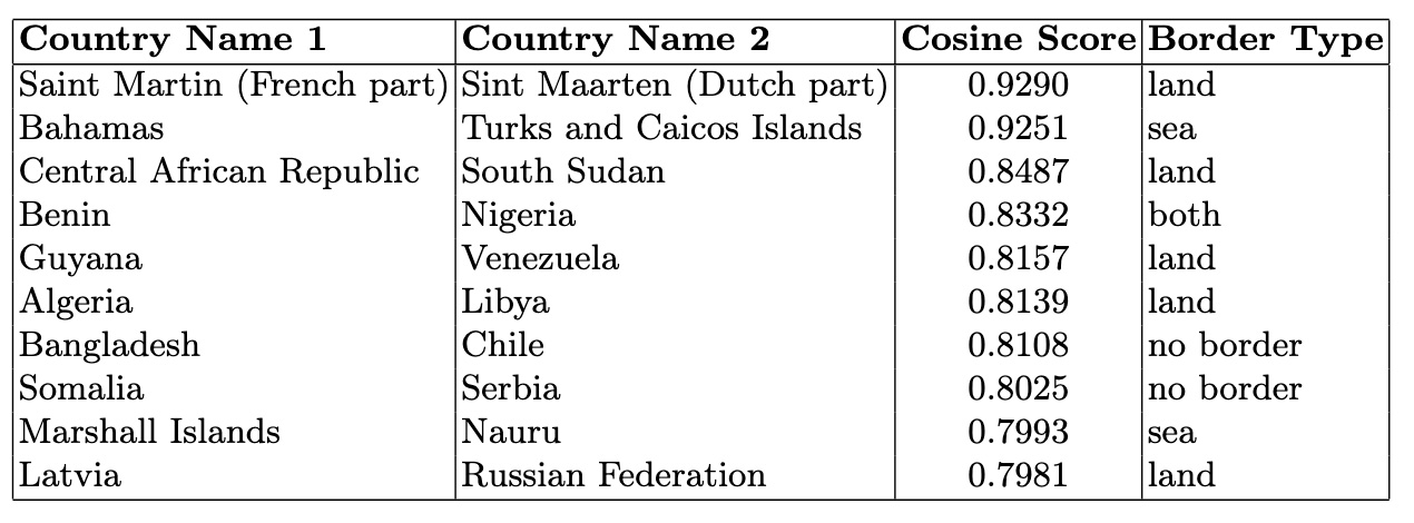
To understand the average relationship strength between countries for each border type, we calculated the mean cosine similarity grouped by "Border Type." This provides an aggregate view of how geographical and feature-based connections correlate across different border categories.
- Cosine Similarity by Border Type:
- Both: 0.429409
- Land: 0.428523
- No Border: -0.009745
- Sea: 0.412243
cosine_similarity_df DataFrame was ordered. By setting it as a categorical variable with the specified order ('both,' 'land,' 'sea,' 'no border'), we maintained a consistent and meaningful arrangement in the boxplot.
The resulting boxplot illustrates the distribution of cosine similarities grouped by border types. This visualization highlights relationships between countries based on their geographic and feature-based connections. The plot's title, labels, and removal of the default subtitle enhance its clarity and readability.
import matplotlib.pyplot as plt
import pandas as pd
cosine_similarity_df['Border Type'] = pd.Categorical(
    cosine_similarity_df['Border Type'],
    categories=['both', 'land', 'sea', 'no border'],
    ordered=True
)
cosine_similarity_df.boxplot(column='Cosine Similarity', by='Border Type')
plt.title('Cosine Similarity by Border Type')
plt.suptitle('')  # Removes the default subtitle
plt.xlabel('Border Type')
plt.ylabel('Cosine Similarity')
plt.show()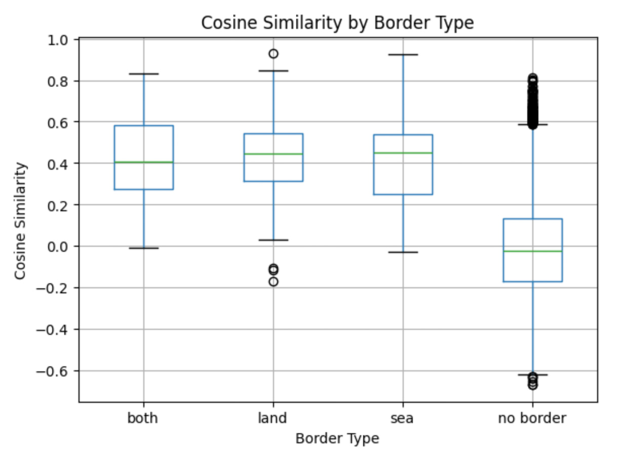
Countries with shared borders, whether by land, sea, or both, tend to have higher cosine similarity, suggesting stronger connections influenced by their geographic proximity. On the other hand, countries without borders show much lower or even negative similarity, emphasizing their distinct differences in socio-economic and other multidimensional features.