Graph Neural Networks for EEG Connectivity Analysis

Introduction

Electroencephalography (EEG) is a widely used non-invasive neuroimaging technique that captures electrical activity in the brain. By recording voltage fluctuations across the scalp, EEG enables researchers to monitor real-time brain activity, providing insights into cognitive processes, mental states, and neurological disorders. It is a valuable tool for understanding how different brain regions coordinate to support functions such as attention, memory, and motor control, making EEG essential for studying neural connectivity.

Traditional methods for analyzing EEG data, such as feature extraction, spectral analysis, and machine learning models like Support Vector Machines (SVM) or Convolutional Neural Networks (CNN), often process channels independently or in predefined groups. While these approaches have achieved moderate success, they struggle to fully model the complex, non-linear spatial and temporal dependencies present in EEG signals. This limitation often results in the loss of crucial information about brain network dynamics.

The graph-like nature of EEG data, where electrode positions can be represented as nodes and interactions as edges, has led to the adoption of Graph Neural Networks (GNNs) for more advanced analysis. GNNs capture the intricate spatial relationships and temporal dependencies in EEG signals, offering a powerful framework for understanding neural dynamics. This capability makes GNNs highly effective for applications such as cognitive state monitoring, emotion recognition, and neurological disorder diagnosis. Recent studies have demonstrated that GNN-based models can provide deeper insights into brain activity compared to traditional methods by revealing subtle connectivity patterns.

Current Study Overview

This study utilizes the publicly available EEG-Alcohol dataset from Kaggle, which includes EEG recordings from subjects exposed to visual stimuli. Trials involved either a single picture stimulus or two picture stimuli, with the latter being either matched (identical) or non-matched (different). This dataset serves as a basis for exploring the impact of alcohol on brain connectivity and cognitive processing.

Building on Prior Work

Our previous studies analyzed this dataset using different methodologies:

• Study 1: Used CNNs and time series analysis to classify EEG signals, showing higher accuracy with Gramian Angular Field (GAF) transformations but limited success in distinguishing Alcoholic and Control groups for single-stimulus trials.


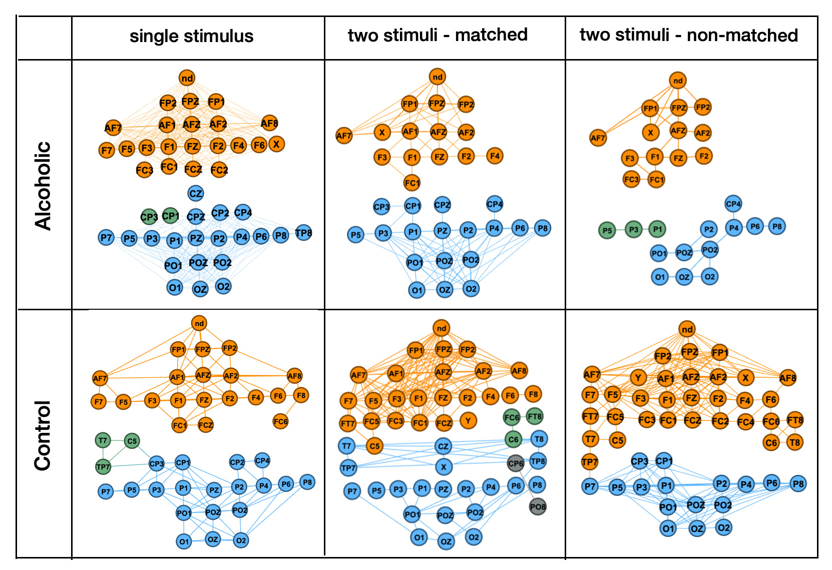
This figure from our previous study shows how connectivity patterns were analyzed using traditional graph mining, revealing stronger and weaker similarities between EEG positions. We found that single-image trials were not effective for distinguishing Alcoholic and Control groups. In this study, we extend these findings by using GNN Link Prediction models.

• Study 2: Employed GNN Graph Classification models, representing each trial as a graph with EEG channels as nodes. While this approach improved classification accuracy, it struggled with single-stimulus trials and highlighted the need for more detailed connectivity analysis.

Building on these findings, this study introduces a unified graph structure where edges represent spatial relationships between EEG channels. This new framework provides a consistent basis for analyzing brain-trial combinations at a granular level, capturing both spatial and temporal dependencies in EEG data.

Significance of the Unified Graph Approach

In contrast to earlier studies that created separate graphs for each trial, this approach integrates all EEG signals into a unified graph structure. Nodes represent EEG channels, while edges reflect spatial proximity, ensuring consistency across analyses. Each trial contributes to a subgraph within the unified structure, capturing both local and global dependencies. The unified graph serves as input for the GNN Link Prediction model, enabling us to detect subtle variations in connectivity across experimental conditions.

By transforming EEG signals into high-dimensional embeddings, this method provides a deeper exploration of spatial and temporal relationships, revealing interactions that conventional techniques could not capture. The study contributes to the growing field of AI-driven neuroscience by offering a versatile framework for analyzing EEG connectivity patterns and improving our understanding of neural dynamics.

Methods

EEG Channel Position Mapping and Graph Construction

This section outlines the process of mapping EEG channel positions in 3D space and constructing an initial graph to capture spatial relationships between the electrodes. The goal was to create a graph where nodes represent EEG channels, and edges reflect their spatial proximity, forming the foundation for subsequent analysis.

EEG Channel Position Extraction

• We loaded the standard EEG montage ('standard_1005') using the mne library.
• Channel positions were retrieved as (x, y, z) coordinates, representing each EEG channel in 3D space.
• Pairwise Euclidean distances between channels were calculated using scipy.spatial.distance, capturing the spatial proximity between electrodes.

Distance Matrix Construction

• The computed distances were used to create a distance matrix that encapsulates the spatial relationships between EEG channels.
• This matrix was formatted into a structured dataset, making it suitable for graph-based modeling.

Minimum Distance Filtering and Graph Creation

• To ensure no channel was isolated, we identified the shortest distance for each channel.
• A distance threshold was applied, defined as the maximum of these minimum distances, to retain only the closest pairs of channels.
• The final graph was constructed with nodes representing EEG channels and edges indicating spatial proximity, ensuring the graph was fully connected for analysis.

Initial EEG Graph Construction

• We built an initial graph representing the spatial configuration of the EEG channels.
• In this graph:
  • Nodes: Represent EEG channels.
  • Edges: Represent spatial proximity between channels.
• Time-series EEG signals for each channel were incorporated as node features, capturing both spatial and temporal dependencies within the EEG data.

Figure 2: An overview of the EEG graph analysis pipeline. The initial graph (left) is built using spatial and temporal EEG data. The GNN Link Prediction model (center) processes the graph to learn node connections, generating embedded vectors (right) that capture complex relationships within the EEG signals for further analysis.

Experiments

Using the EEG-Alcohol dataset from Kaggle, we preprocessed data from 61 EEG channels across multiple trials. The GNN model trained on this graph data demonstrated high accuracy, achieving an 81.45% AUC in distinguishing connectivity patterns between control and alcohol groups. Key differences emerged between experimental conditions, with the control group displaying stronger connectivity in visual processing areas compared to the alcohol group​

Data Source

In our study on brain connectivity, we used the publicly available EEG-Alcohol dataset from Kaggle (Kaggle.com, EEG-Alcohol Data Set, 2017). This dataset contains EEG recordings collected to explore how genetic predisposition to alcoholism might affect neural responses. Each participant was exposed to visual stimuli, either as a single image or two consecutive images. In trials with two images, the stimuli could either be identical (matched) or different (non-matched). The images used were selected from the well-known Snodgrass and Vanderwart picture set, created in 1980, which is commonly used in psychological studies.

The dataset includes EEG data from 8 participants in each group—those with and without alcohol exposure. EEG activity was recorded using 64 electrodes placed across the scalp, capturing brain signals at a high sampling rate of 256 Hz over short, 1-second trials. Due to quality issues in some channels, we focused on data from 61 out of the 64 electrodes, resulting in a total of 61 person-trial pairs included in our analysis.

Our data preparation approach was partly inspired by Ruslan Klymentiev's Kaggle notebook on EEG Data Analysis, which provided a foundation for processing the raw EEG data into a structured format. Building on Klymentiev’s work, we implemented additional transformations to convert these EEG recordings into a structured time series format for each electrode, making the data suitable for graph-based modeling.

To organize the raw sensor data, we categorized it by sensor position and trial number, then created a structured dataset where each row represents a single time point, and each column shows the sensor value from a specific EEG channel at that moment. This transformation was essential for enabling our subsequent graph-based analysis, laying the groundwork for understanding connectivity patterns in the brain. For a more detailed look at our data transformation process, check out our related blog post.

This preprocessing step was crucial as it prepared the dataset for our deeper analysis, allowing us to model brain connectivity patterns effectively. Through this structured data, we could dive into the fascinating world of neural dynamics and uncover insights into how alcohol exposure might influence brain connectivity.

Prepare Input Data for GNN Link Prediction Model

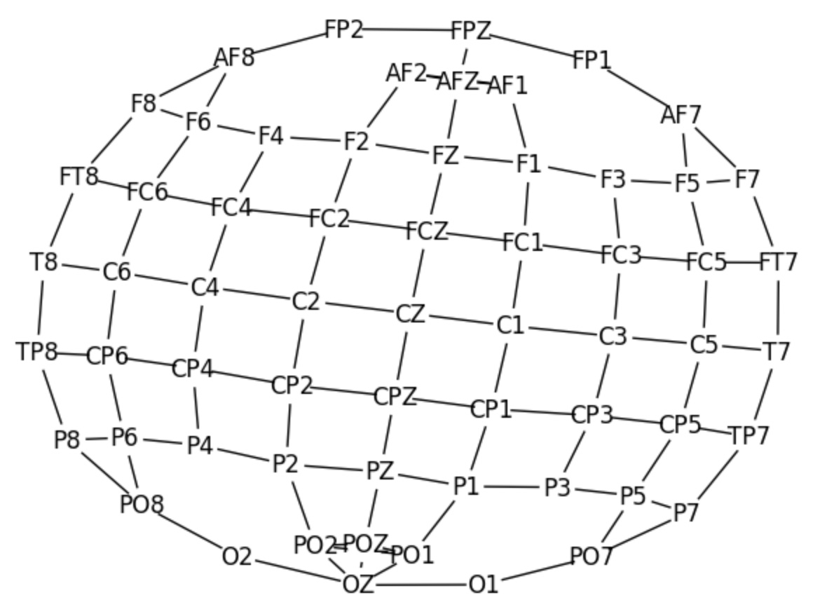
The initial graph structure was created by calculating pairwise Euclidean distances between EEG channels, as outlined in the EEG Channel Position Mapping and Graph Construction subsection of the Methods section. These distances capture the spatial relationships between electrodes based on their physical positions on the scalp. The maximum of the minimum distances between EEG channels was calculated to be 0.038, and to prevent isolated nodes, a slightly higher threshold of 0.04 was used to filter and retain the closest channel pairs. This process resulted in a consistent graph structure with 61 nodes and 108 edges, representing the spatial layout of EEG channels across all subjects and trials. This shared graph provides a uniform topology for all subsequent subject-trial graphs, facilitating comparative analysis.

After establishing the graph structure, we defined graph nodes and their features for each subject-trial combination. Each node corresponds to one of the 61 EEG channels, while node features are derived from the time series signals recorded at these positions during the trials. The data was grouped by type (Alcohol and Control), subject, trial, and channel position, forming structured datasets that capture both spatial and temporal characteristics of the EEG signals. While the spatial configuration of the graph remains constant, node features vary based on each subject and trial, enabling the GNN Link Prediction model to detect connectivity patterns specific to different experimental conditions. For further details on the data preparation process, refer to our related blog post [18].

Data Preparation: Building the Initial Graph Structure

To analyze EEG connectivity patterns effectively, we constructed an initial graph structure that represents the spatial relationships between EEG channels. This process involved calculating pairwise Euclidean distances based on the physical positions of electrodes on the scalp. Using these distances, we created a graph where nodes correspond to EEG channels and edges represent spatial proximity. To ensure no isolated nodes, a distance threshold was set slightly above the maximum of the minimum distances between channels, calculated to be 0.038. A threshold of 0.04 was applied to retain the closest channel pairs, resulting in a connected graph with 61 nodes.

The following Python code demonstrates the steps to build the graph structure, including calculating distances and filtering edges based on the threshold:

import mne
import numpy as np
from scipy.spatial.distance import pdist, squareform

# Load EEG channel positions using MNE's standard montage

montage = mne.channels.make_standard_montage('standard_1005')
pos = montage.get_positions()['ch_pos']
uppercase_pos = {k.upper(): v for k, v in pos.items()}

# Filter positions to retain only the relevant EEG channels

filtered_positions = [ch for ch in positions if ch in uppercase_pos]

len(filtered_positions)
61

The coordinates of the EEG channels were extracted, and a pairwise distance matrix was calculated:

# Extract coordinates for the filtered EEG channels

coordinates = np.array([uppercase_pos[ch] for ch in filtered_positions])
distance_matrix = squareform(pdist(coordinates))

# Calculate pairwise distances and store them in a list

distance_list = []
for i, pos1 in enumerate(filtered_positions):
    for j, pos2 in enumerate(filtered_positions):
        if i != j:  
            distance = distance_matrix[i, j]
            distance_list.append(f"{pos1}, {pos2}, {distance:.6f}")

len(distance_list)
3660

To organize the distances, a DataFrame was created, and the minimum distance for each EEG channel was identified:

import pandas as pd

# Split distance data into a structured DataFrame

split_data = [item.split(", ") for item in distance_list]
distance_df = pd.DataFrame(split_data, columns=["left", "right", "distance"])
distance_df['distance'] = distance_df['distance'].astype(float)

distance_df.head()
# Example output
# left    right    distance
# AF1     AF2      0.038294
# AF1     AF7      0.057702
# AF1     AF8      0.086636
# AF1     AFZ      0.018912
# AF1     C1       0.107897

# Calculate the maximum of the minimum distances

min_distances = {}
for position in set(distance_df['left']).union(set(distance_df['right'])):
    filtered_df = distance_df[(distance_df['left'] == position) | (distance_df['right'] == position)]
    min_distance = filtered_df['distance'].min()
    min_distances[position] = min_distance

max_of_min_distances = max(min_distances.values())

max_of_min_distances
0.038043

Using the calculated maximum of the minimum distances (0.038043), we applied a slightly higher threshold (0.04) to retain only the closest channel pairs. This ensured that the graph remained fully connected, providing a robust structure for subsequent analysis.

This data preparation step was critical for constructing a meaningful graph structure that captures the spatial relationships between EEG channels. By incorporating both node positions and proximity-based edge definitions, this graph provides a solid foundation for analyzing connectivity patterns using Graph Neural Networks.

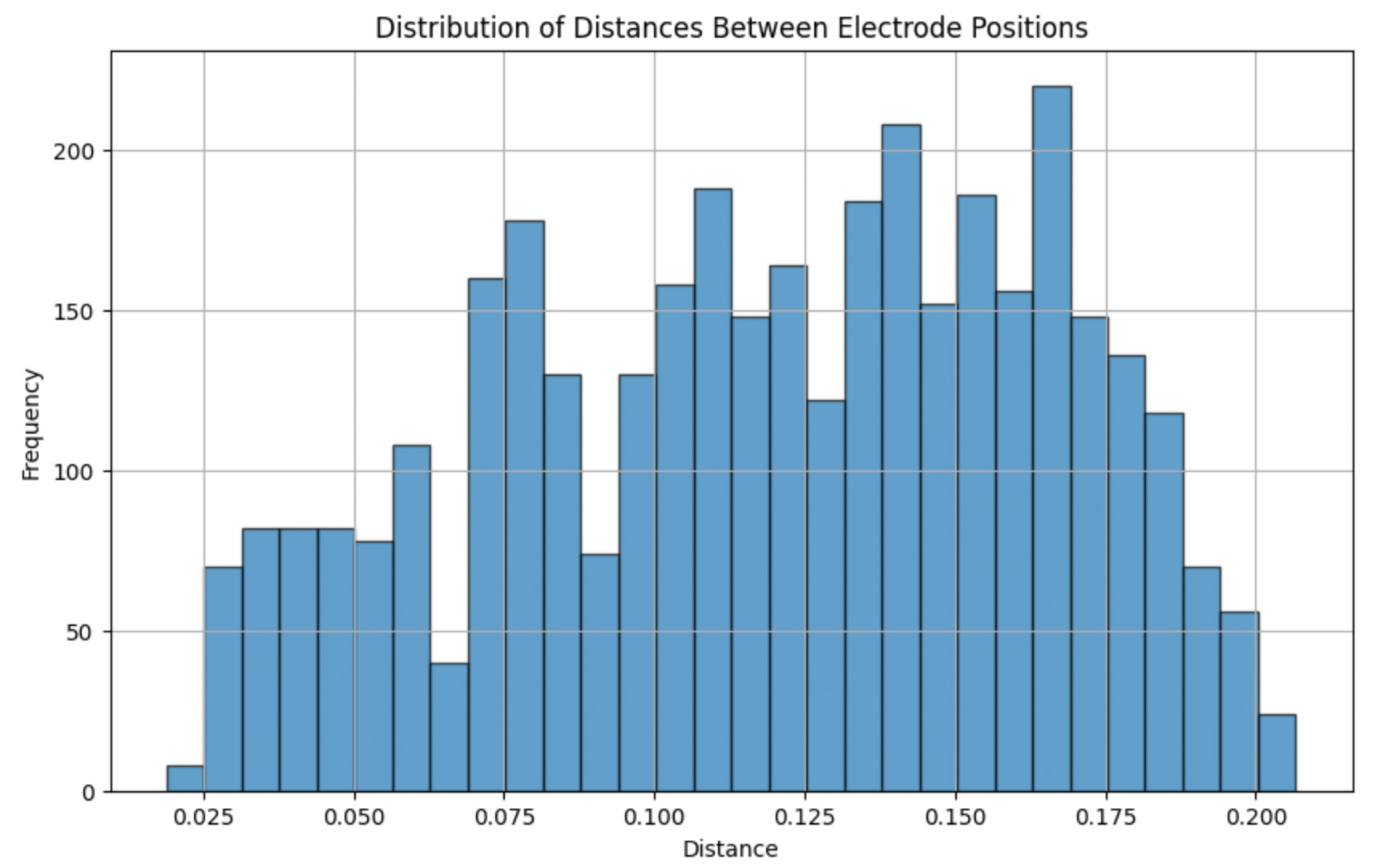
The distribution of distances between electrode positions was analyzed to verify the spatial relationships used for graph construction. Below is a histogram illustrating the distance distribution:

import pandas as pd
import matplotlib.pyplot as plt

plt.figure(figsize=(10, 6))
plt.hist(distance_df['distance'], bins=30, edgecolor='k', alpha=0.7)
plt.title('Distribution of Distances Between Electrode Positions')
plt.xlabel('Distance')
plt.ylabel('Frequency')
plt.grid(True)
plt.show()

# Print basic statistics

print(distance_df['distance'].describe())

Basic statistics of the distances:

• Count: 3660
• Mean: 0.119815
• Standard Deviation: 0.045156
• Min: 0.018912
• Max: 0.206672

Filtered edges below the threshold distance (0.04) were selected to ensure a fully connected graph. The following code demonstrates the construction of the graph:

import networkx as nx

# Filter pairs below the threshold

filtered_pairs = distance_df[distance_df['distance'] < 0.04]

# Create the graph and add edges with weights

G = nx.Graph()
for index, row in filtered_pairs.iterrows():
    G.add_edge(row['left'], row['right'], weight=row['distance'])

# Visualize the graph

pos = nx.kamada_kawai_layout(G)
nx.draw(G, pos, with_labels=True, node_color='white')
plt.show()

The resulting graph represents the spatial relationships between EEG electrodes, as shown in the visualization above. This consistent graph topology is used for all subsequent analyses, with the node features varying based on subject-trial combinations. This approach enables the model to explore dynamic connectivity patterns, providing insights into brain network interactions under different conditions.

For further details on the data preparation and modeling process, refer to our related blog post.

Pre-Training Data Preparation for EEG Graph Neural Network

Following the construction of the initial graph with 61 nodes and 108 edges based on spatial distances between EEG channels, we defined node features for each subject-trial combination. This graph structure provided a uniform topology, enabling the detection of connectivity patterns that varied across different experimental conditions, such as Alcohol and Control groups.

Each node in the graph represents one of the 61 EEG channels, with node features derived from the time series signals recorded during trials. By grouping the data by type (Alcohol and Control), subject, trial, and channel position, we captured both spatial and temporal aspects of the EEG signals. While the graph's spatial configuration remains constant, node features vary across subject-trial combinations, allowing the Graph Neural Network (GNN) Link Prediction model to identify connectivity patterns specific to different conditions.

We started by creating a DataFrame of edges that represents the connections between nodes (EEG channels). This involved combining metadata and filtering edges based on group matching. Here’s the code for constructing the edges:

import pandas as pd
import networkx as nx

# Create an edges DataFrame from the graph's edges

edges = pd.DataFrame(G.edges)
edges.rename(columns={0: 'left', 1: 'right'}, inplace=True)

# Separate feature and metadata columns

values = rawData.iloc[:, 6:262]
metavalues1 = rawData.iloc[:, 0:6]
metavalues2 = rawData.iloc[:, 262:]
metavalues = pd.concat([metavalues1, metavalues2], axis=1)

# Drop unnecessary metadata columns and merge with edges

metaData = metavalues.drop(['trial', 'type', 'match', 'name', 'channel'], axis=1)
edges_left = metaData.merge(edges, left_on='positionIdx', right_on='left').drop('position', axis=1)
edges_left.rename(columns={'index': 'left_index'}, inplace=True)
edges_right = edges_left.merge(metaData, left_on='right',
   right_on='positionIdx').drop('position', axis=1)
edges_right.rename(columns={'index': 'right_index'}, inplace=True)

# Filter edges by group matching and reset index

filtered_edges = edges_right[edges_right['group_x'] == edges_right['group_y']]
edges_final = filtered_edges.drop(['group_y'], axis=1).reset_index(drop=True)
edges_final['index_final'] = edges_final.index  # Add final index as a column

# Create the final NetworkX graph from the processed edges DataFrame

G = nx.from_pandas_edgelist(edges_final, source='left_index', target='right_index')

After defining the edges and nodes, we used the Deep Graph Library (DGL) to convert the NetworkX graph into a DGL graph. We then added the node features (time series signals) as tensors, which the model will use to analyze connectivity patterns. Here’s the code for preparing the DGL graph and adding features:

import dgl
import torch

# Convert NetworkX graph to DGL graph

g = dgl.from_networkx(G)

# Convert EEG time series data to a tensor and add it as node features

values = rawData.iloc[:, 6:262]
features_tensor = torch.tensor(values.values, dtype=torch.float32)
g.ndata['feat'] = features_tensor

# Display the graph summary

g
Graph(num_nodes=3721, num_edges=13176,
      ndata_schemes={'feat': Scheme(shape=(256,), dtype=torch.float32)}
      edata_schemes={})

This data preparation stage established a robust graph-based representation of EEG data, where each node (EEG channel) has unique features based on time series signals across trials. The resulting graph, with 3721 nodes and 13176 edges, serves as input to the GNN model, allowing it to explore complex connectivity patterns across experimental conditions. This setup lays the groundwork for effective pre-training and connectivity analysis.

For more information on the data preparation process and detailed GNN modeling steps, refer to our related blog post.

Train the Model

We utilized the GraphSAGE link prediction model, implemented with the Deep Graph Library (DGL), to train our model on the EEG graph data. GraphSAGE employs two layers to aggregate information from neighboring nodes, enabling the model to capture complex connectivity patterns and interactions between EEG channels.

• Total Nodes: 3,721
• Total Edges: 13,176
• Node Feature Size: 256

The model’s performance was evaluated using the Area Under the Curve (AUC) metric, achieving an accuracy of 81.45%. This high AUC score demonstrates the model’s effectiveness in predicting connectivity patterns and capturing the underlying signal dependencies within the EEG data.

We implemented our model using code from the tutorial "Deep Graph Library (DGL): Link Prediction Using Graph Neural Networks," published in 2018. This resource provided a foundational framework for building and optimizing our GraphSAGE-based link prediction model.

EEG Connectivity Analysis: GNN Link Prediction and Statistical Calculations

The foundation of our connectivity analysis stems from the results of a Graph Neural Network (GNN) link prediction model. This model generates a matrix, h, where each row represents an embedded vector corresponding to a graph node. In our context, these nodes represent EEG channels, and the embedded vectors capture the spatial and temporal relationships between signals from different brain regions.

These embeddings provide a powerful, compressed representation of connectivity patterns, allowing us to measure the relationships between nodes through cosine similarity.

To evaluate the strength of connections between EEG nodes, we calculated pairwise cosine similarity scores between their embedded vectors. Cosine similarity measures the cosine of the angle between two vectors, producing a value between -1 (completely opposite) and 1 (completely identical).

Below is the PyTorch-based implementation for calculating cosine similarity:

import torch

# Define a function to calculate cosine similarity using PyTorch

def pytorch_cos_sim(a: torch.Tensor, b: torch.Tensor):
    return cos_sim(a, b)

def cos_sim(a: torch.Tensor, b: torch.Tensor):

# Ensure inputs are PyTorch tensors

    if not isinstance(a, torch.Tensor):
        a = torch.tensor(a)
    if not isinstance(b, torch.Tensor):
        b = torch.tensor(b)

# Adjust dimensions for single-row tensors

    if len(a.shape) == 1:
        a = a.unsqueeze(0)
    if len(b.shape) == 1:
        b = b.unsqueeze(0)

# Normalize the vectors

    a_norm = torch.nn.functional.normalize(a, p=2, dim=1)
    b_norm = torch.nn.functional.normalize(b, p=2, dim=1)

# Compute cosine similarity

    return torch.mm(a_norm, b_norm.T)

# Example usage: compute cosine similarity for matrix `h`

cosine_scores = pytorch_cos_sim(h, h)

Statistical Analysis Using Self-Join Cosine Similarity

Once the cosine similarity matrix (cosine_scores) is computed, we perform statistical calculations by grouping the data and applying self-join operations. This allows us to analyze the pairwise connectivity patterns within specific experimental groups (e.g., Alcohol and Control) and conditions (e.g., Single Stimulus, Two Stimuli).

The self-join operation systematically computes pairwise statistics within each group, focusing on unique connections between EEG channels. Below is the implementation:

group_scores = []

# Iterate over each unique group in the 'group' column

for group_idx in metaRawData['group'].unique():

# Filter rows that belong to the current group

    group_data = metaRawData[metaRawData['group'] == group_idx]

# Extract `type`, `match`, and `name` for the group (assuming they are the same for the group)

    group_type = group_data['type'].iloc[0]
    group_match = group_data['match'].iloc[0]
    group_name = group_data['name'].iloc[0]

# Get the indices of the rows for the current group

    group_indices = group_data.index

# Calculate self-join cosine similarity within the group

    for i, row_i in enumerate(group_indices):
        position_i = metaRawData.loc[row_i, 'position']

# Start from the next index to avoid duplicate pairs (i, j) and (j, i)

        for j, row_j in enumerate(group_indices[i+1:], start=i+1):
            position_j = metaRawData.loc[row_j, 'position']

# Retrieve cosine similarity score from cosine_scores array

            cos = cosine_scores[row_i][row_j].item()

# Append the results to the list

            group_scores.append({
                'group': group_idx,
                'type': group_type,
                'match': group_match,
                'name': group_name,
                'position_i': position_i,
                'position_j': position_j,
                'left_idx': row_i,
                'right_index': row_j,
                'cosine_similarity': cos
            })

The result of this process is a structured dataset where each row represents a unique connection between two EEG channels, along with the computed cosine similarity and group-level metadata. An example entry might look like this:

{
    "group": "Alcohol",
    "type": "Experimental",
    "match": "Two Stimuli - Matched",
    "name": "Subject 1",
    "position_i": "Cz",
    "position_j": "Pz",
    "left_idx": 5,
    "right_index": 10,
    "cosine_similarity": 0.76
}

Key Insights and Applications

• Condition-Wise Connectivity Analysis: Aggregating cosine similarity scores allows us to compare connectivity strength between experimental groups (e.g., Alcohol vs. Control) under various conditions (e.g., Single Stimulus, Two Stimuli).
• Node-Level Connectivity Patterns: The position_i and position_j fields enable spatial mapping of connectivity patterns across the brain.
• Group Comparisons: By grouping the results, we can identify statistically significant differences in connectivity patterns between conditions.

The combination of GNN embeddings, cosine similarity, and statistical grouping enables a robust and scalable approach to analyzing EEG connectivity. By leveraging self-join matrices, we quantify pairwise relationships between EEG channels, uncovering patterns that provide valuable insights into the neural effects of experimental conditions such as alcohol exposure.

Interpreting Model Results

Condition-wise Analysis of Cosine Similarities

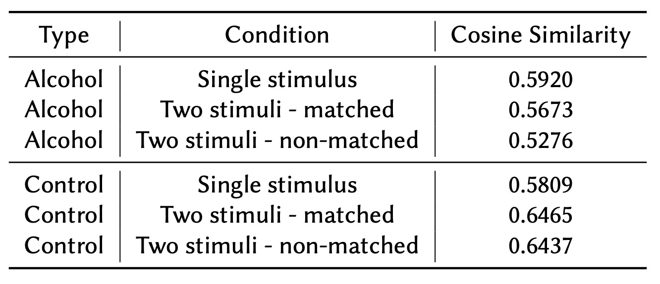
To compare connectivity patterns between the Alcohol and Control groups, we computed the average cosine similarities from the embedded vectors generated by the model. These cosine similarities represent the strength of connectivity between brain regions, with higher values indicating stronger connections. The computed values were aggregated by condition type and match status to assess differences across the experimental groups.

As shown in Table 1, the ‘Single stimulus’ condition revealed minimal differences between the Alcohol and Control groups. This finding aligns with results from our previous studies [2, 3]. Since the ‘Single stimulus’ condition did not show significant variation in connectivity patterns, it was excluded from further analysis.

We instead focused on the ‘Two stimuli - matched’ and ‘Two stimuli - non-matched’ conditions, where clearer distinctions between the groups were observed:

• Alcohol group: Average cosine similarity of 0.546.
• Control group: Average cosine similarity of 0.645.

The higher average cosine similarity in the Control group suggests stronger overall connectivity compared to the Alcohol group. This finding may reflect differences in the efficiency or robustness of neural communication between the two groups. These variations could be indicative of the impact of alcohol on brain connectivity.

In the following sections, we will delve deeper into these patterns at the node level, highlighting specific regions of the brain with both high and low signal correlations between the groups.

This table shows average cosine similarities by condition and group:

Strongly Connected Positions

Our analysis utilized a GNN Link Prediction model to explore the EEG connectivity patterns in both the Alcohol and Control groups. This model was specifically designed to capture the intricate spatial relationships and temporal dependencies present in EEG data. By analyzing connectivity patterns at a granular level, the GNN Link Prediction model provided critical insights into how different brain regions interact under various experimental conditions.

The GNN Link Prediction model generated embedded vectors, which were used to calculate edge weights based on the initial graph structure. Node-level cosine similarities were then computed by combining left and right node positions, grouping them by type and position, and averaging the values to evaluate overall connectivity strength.

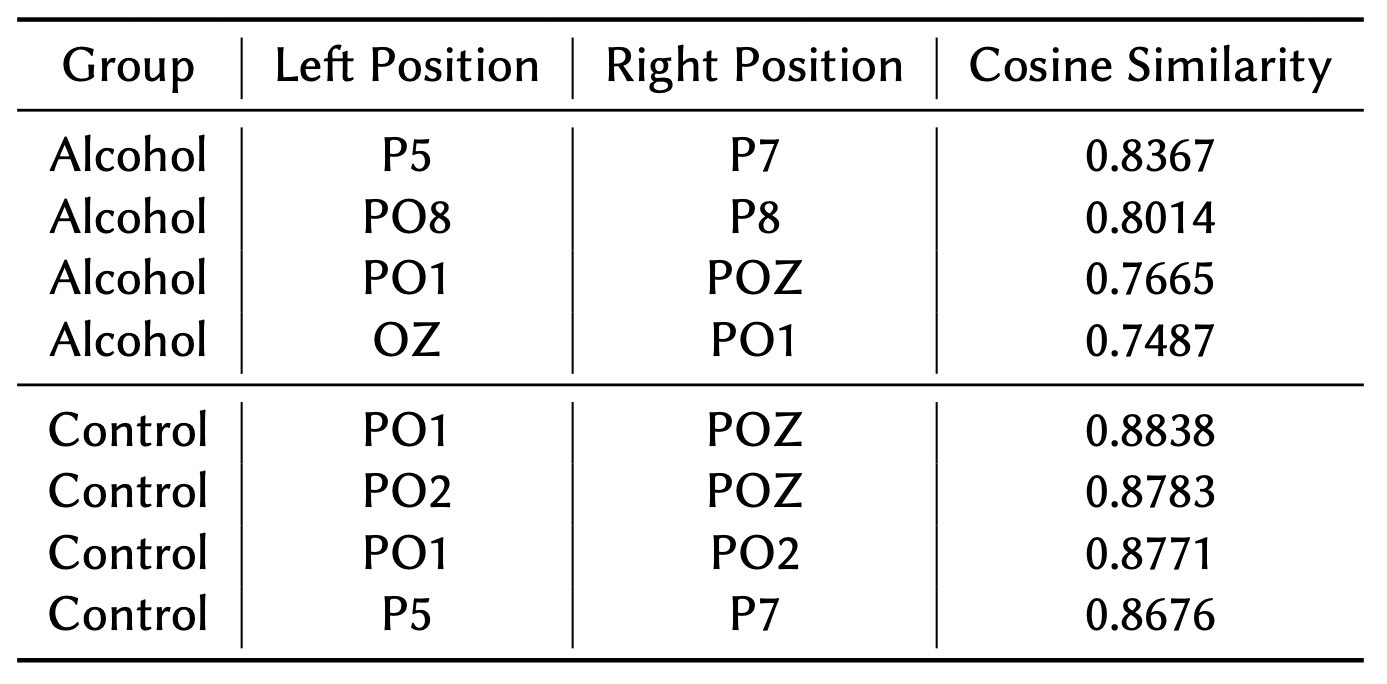
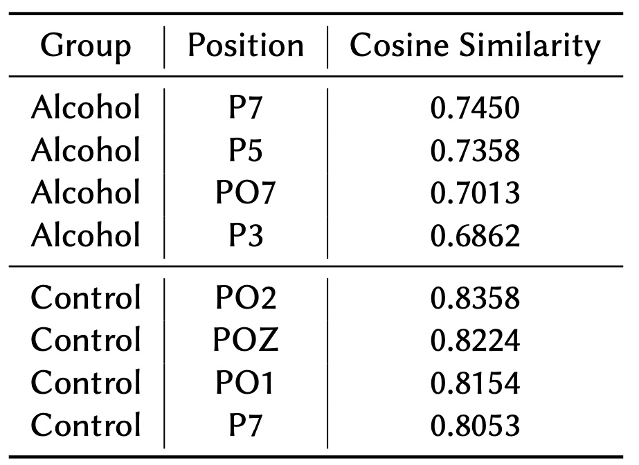
Tables 2 and 3 highlight the top highly connected node pairs and nodes, respectively. In the Control group, the strongest connections are concentrated in the occipital and parietal regions. These regions play a vital role in visual processing and sensory integration, showcasing a stable and efficient brain network organization. The occipital region's dominance in the Control group suggests healthy neural patterns without significant disruptions. This enables consistent and efficient communication within the brain, particularly in areas essential for interpreting visual input.

On the other hand, the Alcohol group displays more disruptions, characterized by lower overall connectivity values. Although connections are observed in the parietal and occipital regions, they are weaker compared to the Control group. This indicates a less organized and consistent brain network in the Alcohol group, likely reflecting the effects of alcohol on neural connectivity. Interestingly, the parietal region's dominance in the Alcohol group might suggest a compensatory mechanism, where the brain attempts to enhance connectivity in regions responsible for sensory processing and spatial awareness to counterbalance alcohol-induced disruptions.

Table 2 highlights the top connected node pairs based on cosine similarity for the Alcohol and Control groups. The analysis reveals that the Alcohol group exhibits strong connectivity in the parietal and occipital regions, which are associated with sensory processing and spatial awareness. However, the Control group demonstrates even stronger connections within the occipital area, a region crucial for visual processing and sensory integration.

These findings suggest that the Control group has a more stable and efficient brain network organization, enabling robust communication between regions involved in visual and sensory information processing. In contrast, the Alcohol group's connectivity, while present, appears less stable, potentially reflecting the impact of alcohol on neural communication pathways.

Table 3 showcases the nodes with the highest cosine similarity values for both the Alcohol and Control groups. In the Alcohol group, the strongest connectivity is observed in the parietal region, suggesting a focus on regions responsible for sensory processing and spatial awareness. This pattern could indicate a compensatory mechanism in response to disruptions caused by alcohol.

Conversely, the Control group shows dominance in the occipital region, which reflects consistent and efficient neural communication critical for interpreting visual information. This occipital region dominance highlights the Control group's more organized and robust brain network, supporting efficient sensory and visual information processing. The contrast between the two groups underscores differences in how the brain processes sensory and visual stimuli under varying conditions.

Weakly Connected Positions

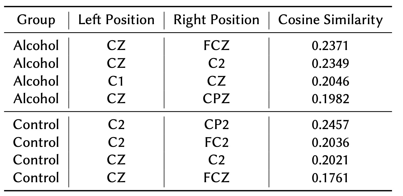
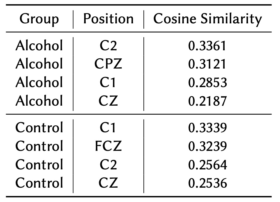
As shown in Tables 4 and 5, the nodes and node pairs with the lowest cosine similarity values for both the Alcohol and Control groups are concentrated in the central brain regions, such as CZ, C1, and C2. These regions are primarily associated with motor functions and are not expected to exhibit high connectivity in trials focused on visual stimuli. This finding aligns with the task's emphasis on visual processing rather than motor activity.

In the Control group, these motor-related regions display low connectivity, which is consistent with the visual nature of the task. However, in the Alcohol group, the connectivity in these regions is even weaker, indicating that alcohol exposure may lead to broader disruptions across brain networks, even in areas not directly involved in the experimental task. This suggests that alcohol may impair not only task-relevant connectivity but also overall neural network stability.

Table 4 highlights node pairs with the lowest cosine similarity values in both the Alcohol and Control groups. These weakly connected regions are particularly concentrated in central areas associated with motor function. While both groups show reduced connectivity in these regions, the Alcohol group exhibits more pronounced disruptions, indicating a broader impact of alcohol on neural networks.

Table 5 identifies individual nodes with the lowest cosine similarity values in both groups, primarily located in central regions such as CZ, C1, and C2. The Control group maintains slightly higher connectivity in these areas, aligning with the task's visual focus. In contrast, the Alcohol group demonstrates more pronounced disruptions, further reflecting the potential impact of alcohol on overall brain network stability.

Graphical Representation of High and Low Connectivity Nodes

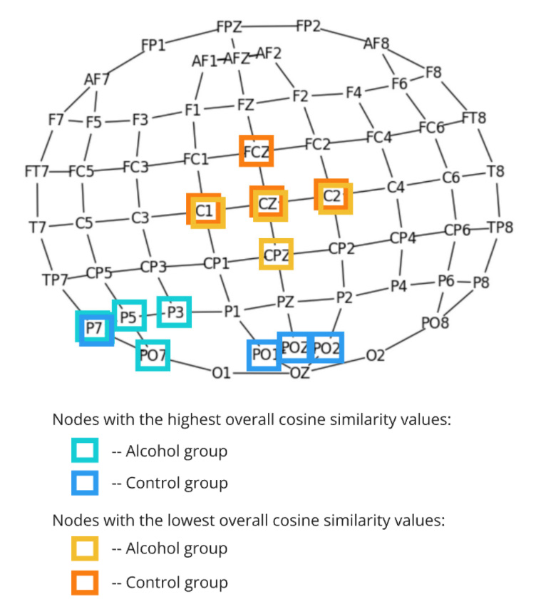
The figure displays a topographical map of EEG channels, highlighting nodes based on their overall cosine similarity values for the Alcohol and Control groups. Nodes with the highest connectivity are shown in turquoise for the Alcohol group and in blue for the Control group, while those with the lowest connectivity are represented in yellow for the Alcohol group and orange for the Control group. This visualization offers a clear comparison of connectivity patterns, identifying regions of stronger and weaker signal correlations.

In the Control group, the high-connectivity nodes are primarily located in the occipital region, which is responsible for visual processing. This stable neural interaction is expected during visual trials, indicating efficient brain network organization in response to visual stimuli. In contrast, the Alcohol group exhibits stronger connections in the parietal region, with fewer occipital nodes involved. This shift in connectivity may indicate how alcohol alters brain activity, possibly disrupting normal visual processing and causing compensatory activity in other regions.

Both groups demonstrate low connectivity in the central region, which is typically linked to motor and sensorimotor processing. The lower activity in these areas during visual trials suggests they are not heavily engaged, aligning with their expected limited role in visual perception and processing tasks.

In Conclusion

This study highlights the potential of GNN Link Prediction models to uncover subtle variations in EEG connectivity, providing a deeper understanding of neural dynamics. By developing a unified graph structure based on spatial distances between EEG electrodes, we successfully applied these models to analyze and interpret brain connectivity patterns in both Alcohol and Control groups.

Our findings reveal that GNN Link Prediction models offer unique insights into connectivity patterns that traditional methods might miss. In the Control group, high-connectivity nodes were predominantly found in the occipital region, which is crucial for visual processing, reflecting stable and efficient neural responses. In contrast, the Alcohol group exhibited stronger connectivity in the parietal region, suggesting compensatory mechanisms to address disruptions caused by alcohol exposure. This shift highlights how alcohol may alter typical brain activity, particularly in regions linked to sensory and cognitive functions.

Beyond EEG analysis, this framework is adaptable to other types of time series data, making it a versatile tool for studying connectivity patterns and uncovering underlying physiological dynamics. By integrating AI with neuroscience, this work demonstrates how GNN Link Prediction models can enhance our understanding of brain connectivity and open new avenues for research and clinical applications.

Workshop

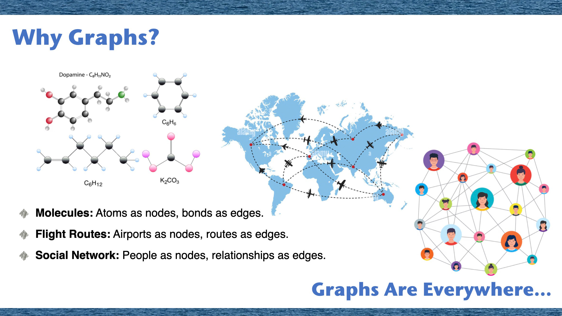
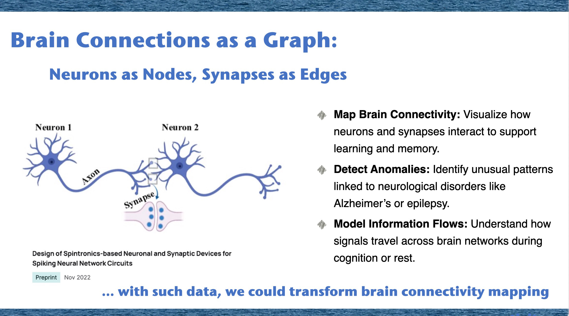
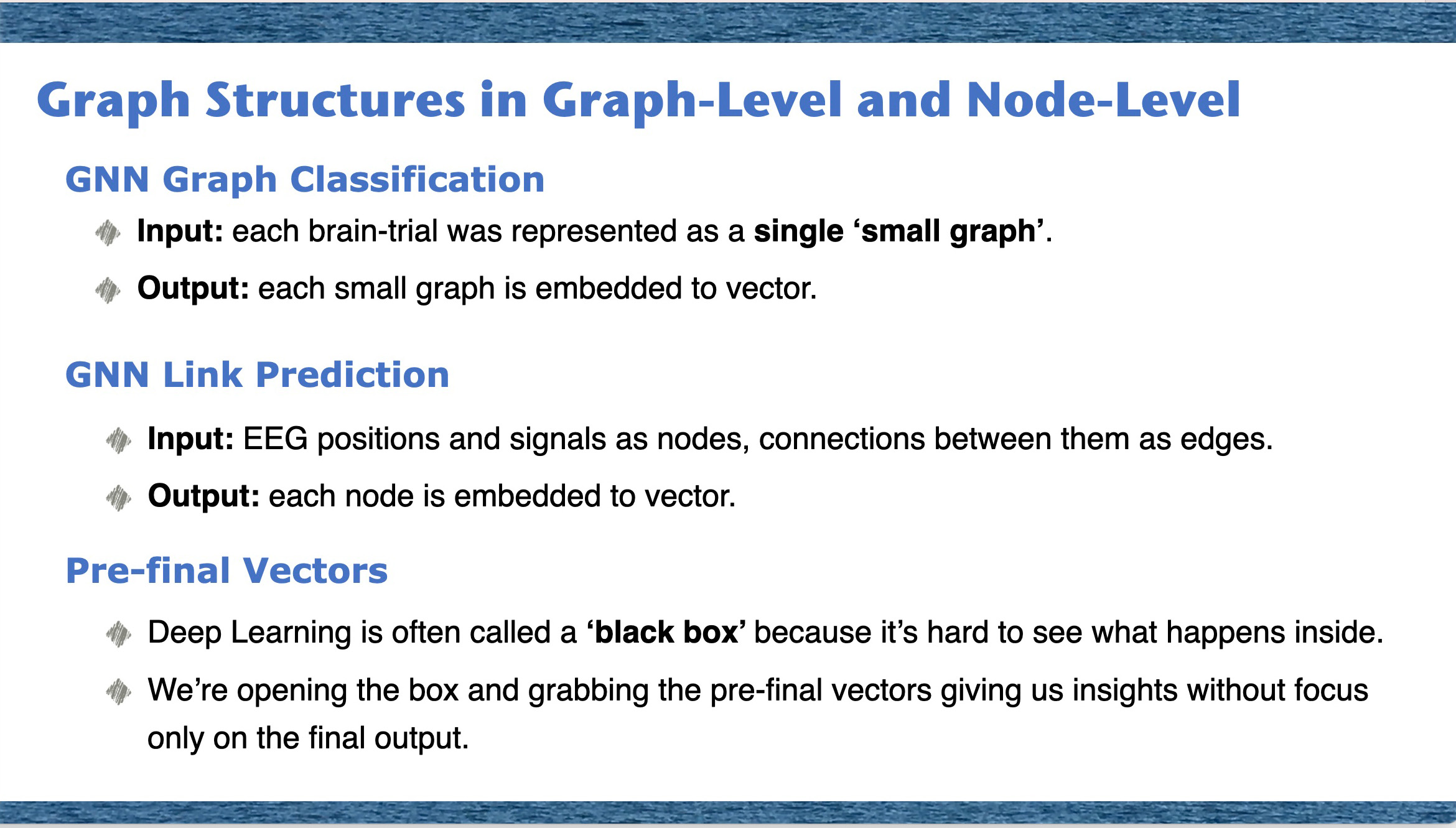
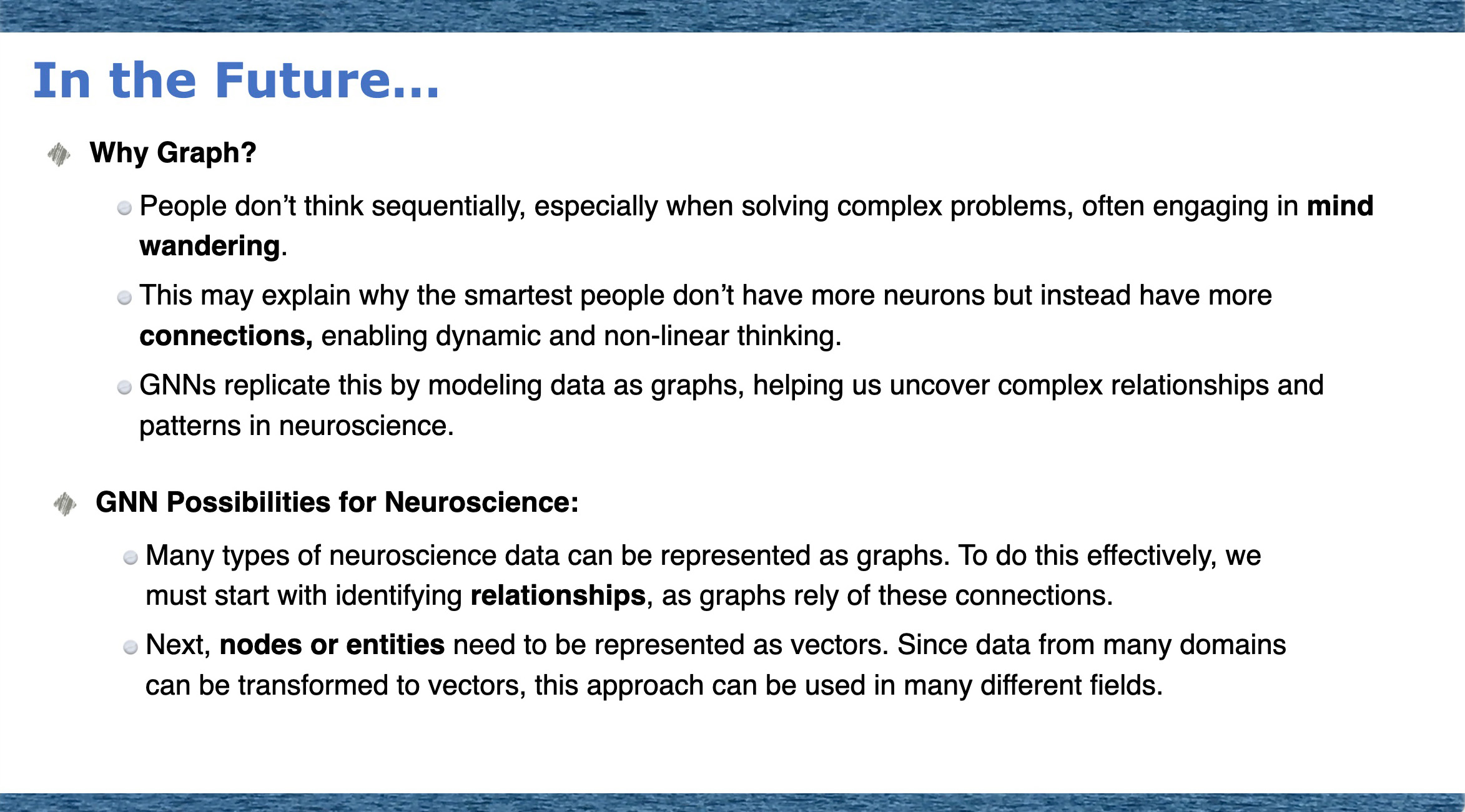
This study was presented in “2024 International Workshop on Artificial Intelligence for Neuroscience” - workshop in Alicante, Spain on November 26, 2024. Here are some slides from the presentation that are not in this poster.

We started with explaining people that graphs are everywhere in our lives. They represent molecules in chemistry, roads in navigation, and even our social networks like Facebook as molecule graphs, traffic graph, and social network graph.

Then we showed that perhaps the most important graph of all is the one inside us: the network of neurons and synapses that forms our brain and for neuroscience, understanding graphs is key to unraveling how our brains process information, learn, and adapt.

Then we introduced deep learning history, how GNN was created and what is the most important to know about GGN models.

Finally, we discussed why for neuroscience graph thinking is really important and how neuroscientists can start thinking in that direction.

• ← Previous Post