Semantic Graphs for Communication Networks
In this project, we move beyond simple “who emailed whom” graphs and build a semantic graph of communication. Instead of treating edges as raw message counts, we create nodes for individual interactions (who wrote to whom, with what text), enrich them with transformer-based text embeddings, and use a GNN link prediction model to learn which interactions are genuinely related. This text-enriched graph lets us recompute centrality and see a different set of key players: not just the loudest senders, but the quiet connectors who bridge topics and conversation clusters—hidden connectors that a plain traffic graph would never reveal.
Conference & Workshop
The work “Multi-Layer Graph Analysis for Text-Driven Relationships Using GNN Link Prediction” was presented at the MLH 2024 – Mining and Learning with Hypergraphs workshop, co-located with ECML-PKDD 2024, in Vilnius, Lithuania, on 13 September 2024. The contribution appears in the non-archival online workshop program and is available via the MLH 2024 website.
Multi-Layer Graph Analysis for Communication Networks
Analyzing complex graphs can be quite challenging, especially when the whole is greater than the sum of its parts. To address these challenges, we dive into the Enron email dataset, using its rich information to create a strong multi-layer graph analysis framework. We start by building a foundational graph layer where email addresses are the nodes and email exchanges form the edges. This layer gives us a clear picture of the communication network, showing the direct interactions between individuals within the dataset. Building upon this, we introduce a second graph layer that goes deeper into the content of these communications. Here, each interaction is represented as a node in the form of triplets—comprising the sender, receiver, email subject, and body. Edges in this layer signify communication chains, illustrating how discussions and information flow within the network. To extract meaningful patterns from the textual content, we transform these triplet nodes into vectors using a transformer model. This transformation captures the semantic nuances of the email content. Following this, a Graph Neural Network (GNN) Link Prediction model is applied to these vectors. The model identifies potential links within the graph based on semantic similarity and structural patterns. The output vectors from the GNN Link Prediction model, which capture both the semantic content and the graph structure, help us create a third graph layer. In this layer, nodes represent pairs of emails with high cosine similarities, forming a network that highlights strong semantic connections. This third graph layer is key to identifying influencers within the network, revealing individuals who play important roles in spreading information. It also gives us a better understanding of engagement dynamics, showing how interactions evolve and spread across the network. By using this multi-layer approach, we provide a comprehensive framework for analyzing complex textual interactions within graph structures. This method not only offers deeper insights into network dynamics but also improves our ability to identify key influencers, ultimately enhancing our understanding of intricate communication networks.Introduction
Graphs are powerful tools for representing complex relationships, with each level building on the previous one’s capabilities and efficiency. Think of atoms forming molecules with unique properties, molecules creating cells with essential functions, and cells building organs with specialized roles. However, as graphs become more intricate, analyzing them becomes increasingly challenging. Complex system analysis can be approached both top-down and bottom-up. In this study, we introduce a bottom-up method for analyzing graph layers built on text-driven relationships. This approach captures intricate details and emergent properties from foundational elements upwards. For example, imagine a bipartite graph with individuals on one side and movie narratives on the other. Relationships in this graph are defined by shared interests in particular movies. By exploring the narrative elements in recommender systems, we can uncover complex relationships that go beyond merely identifying pairs or groups of people with common movie interests. Another example is influence networks in social media, where nodes represent users and directed edges signify interactions such as likes, comments, or shares. By examining the content of posts and interactions, we can uncover text-driven relationships that reveal influence patterns and topics of interest. This approach helps us understand the dynamics of influence and engagement within the social media ecosystem. In a prior study 'Rewiring Knowledge Graphs by Graph Neural Network Link Predictions' (2023), we focused on rewiring text-based knowledge graphs through the use of GNN link prediction models, specifically targeting semantic knowledge graphs built from text documents. We utilized GNN link prediction techniques to modify these graphs, revealing hidden connections between nodes. In another study 'Uncovering Hidden Connections: Granular Relationship Analysis in Knowledge Graphs' (2024), we also applied GNN link prediction models to semantic knowledge graphs to uncover hidden relationships within a detailed vector space. We focused on identifying 'graph connectors' that expose deeper network structures and used graph triangle analysis to delve into complex interactions. The Enron email corpus provides a valuable opportunity to explore the potential of text-enhanced knowledge graphs in uncovering hidden patterns within organizational communication. By focusing on direct interactions and using transformer models for text embedding, we lay the groundwork for a knowledge graph that better captures the complexity of real-world relationships. Our findings highlight the significant impact of incorporating textual data and GNN Link Prediction in knowledge graph analysis. This approach provides a more complete view of how entities interact, helping us understand complex networks better. As we continue to refine these methods, the potential for uncovering new insights in data-rich environments seems limitless, opening up exciting possibilities for future research.Key Methodologies of Our Study
Architecture Pipeline
Our architecture pipeline for the multi-layer graph approach begins with raw data processing and follows to link prediction model: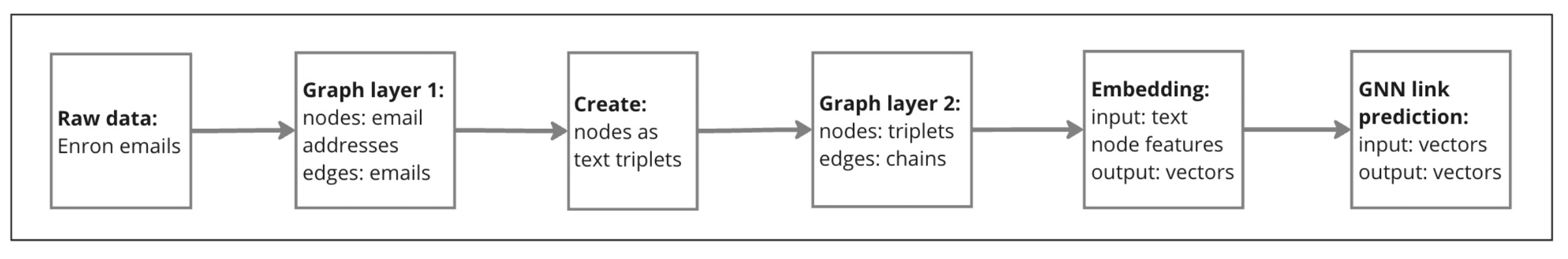
- Raw Data: The initial dataset includes attributes such as ‘from’, ‘to’, ‘body’, and ‘time’.
- Initial Graph Layer: Email addresses are depicted as nodes connected by edges representing email exchanges.
- Transformation to Triplet Nodes: Email exchanges are converted into triplets (from, to, email body).
- Second-Layer Graph Construction: Triplet nodes form edges based on communication chains (to-to connections).
- Node Embedding: Embedding node features to vectors.
- GNN Link Prediction: The GNN model is applied, transforming triplet nodes into vectors.
After GNN Link Prediction model training, we will examine structural changes in the network to uncover key influencers.
Transformation Process from Initial Graph to Second-Layer Graph
The process begins with constructing the initial graph layer, where email addresses are depicted as nodes connected by edges representing email exchanges, as shown in the picture. Each email exchange is then converted into triplets consisting of 'from', 'to', and the email's subject and body. Subsequently, a second-layer graph is constructed where these triplet nodes form edges based on communication chains ('to-to' connections), as illustrated in the picture.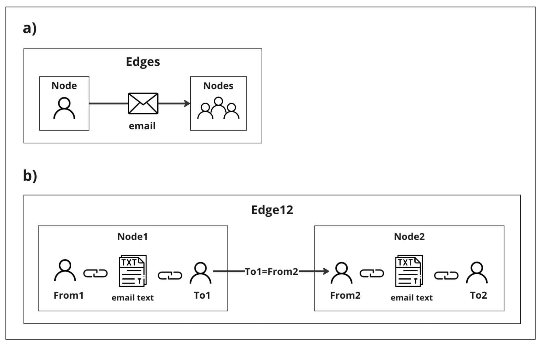
Node Embedding
To translate text into vectors, we will use the 'all-MiniLM-L6-v2' transformer model from Hugging Face. This sentence-transformer model efficiently maps text into 384-dimensional vectors. This process transforms sentences into dense vectors, preserving their semantic content for machine learning applications. This embedding step is crucial, ensuring the text is suitably prepared for deep learning analyses, including GNN link prediction, by capturing the nuanced meanings in a format compatible with our algorithms.Training the GNN Link Prediction Model
After setting up the nodes, we refine the graph with GNN Link Prediction to uncover detailed interactions. By examining the graph’s structure and node details, we reveal previously hidden connections, enhancing the graph’s depth and utility for analysis. We use the GraphSAGE link prediction model, which generates node embeddings based on attributes and neighbors without retraining. Our study employs a GNN Link Prediction model from the Deep Graph Library (DGL), with two GraphSAGE layers. This approach improves node representation by combining details from nearby nodes and discovering hidden connections in the Enron email dataset. The output vectors from this model can be used for further analysis, and we will showcase this in our 'Experiments' section.Experiments Overview
Data Source
Our main data source is the Enron email corpus, a comprehensive collection of emails exchanged among executives of the Enron Corporation. This dataset, freely available to the public, captures a wealth of corporate communications, offering a deep dive into the intricacies of a complex organizational network. Its rich detail makes it an excellent resource for our knowledge graph analysis, shedding light on the dynamics of corporate interactions. The Enron email corpus is hosted on Kaggle, providing easy access for those looking to conduct detailed analyses of the dataset. For further information or to explore the dataset yourself, visit Kaggle's Enron Email Dataset.Input Data Preparation
Our study starts with building a graph using the Enron email dataset from the year 2000, focusing on internal communications by selecting emails sent from @enron.com addresses. We aimed to analyze direct email exchanges between individuals, excluding group emails to ensure a clear and focused analysis. For the graph’s nodes, we merged the 'From', 'To', 'Subject', and 'Body' fields of each email into a single text unit, as illustrated in the picture. This method ensures that each node fully represents an individual email conversation, including all its context and specifics. To link these nodes in the graph, we connected emails that had either the same sender or recipient, indicating a direct line of communication between parties. This setup accurately mirrors how communication unfolded within Enron, revealing the network’s detailed structure and the rich interplay of relationships among employees.Constructing Layer Graphs from Enron's 2000 Email Corpus
Our investigation begins by creating a knowledge graph derived from the Enron email dataset, specifically focusing on the year 2000. Our selection criteria were emails exchanged internally, identifiable through @enron.com addresses, allowing us to concentrate on direct communications between individual employees while excluding group emails for a more targeted analysis.Node Creation in the Knowledge Graph
To form the nodes of our knowledge graph, we combined the 'From', 'To', 'Subject', and 'Body' of each email into a unified text representation. This approach ensured that each node captured the entirety of an email exchange, preserving both the context and the details of the conversation. Concatenate 'From', 'To', 'Subject', and 'body' columns with '^' betweendf['emailText'] =
df[['From','To','Subject', 'body']]
.apply(lambda row: ' ^ '.join(row.values.astype(str)), axis=1)unique_emails = pd.concat([df['From'], df['To']]).unique()
email_index = pd.Series(index=unique_emails, data=range(len(unique_emails)), name='emailIdx')
df['FromIdx'] = df['From'].map(email_index)
df['ToIdx'] = df['To'].map(email_index)
emailFromTo=df[['FromIdx','emailTextIdx','emailText', 'ToIdx']]
emailFromTo.tail()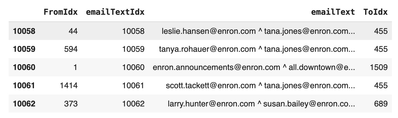
Linking Nodes in the Knowledge Graph
In establishing connections within the knowledge graph, we linked emails sharing common senders or recipients, thereby reflecting a direct communication pathway between entities. This method provided an accurate reflection of how interactions occurred within Enron, uncovering the intricate structure of the network and the dynamic web of relationships between employees. Self-join emailFromTo table to create edges:df=emailFromTo
joined_df =
df.merge(df, left_on='ToIdx', right_on='FromIdx', suffixes=('_left', '_right'))
df2 = joined_df.query('FromIdx_left != ToIdx_right')
dfLeft = em2text2em[['emailText_left', 'emailTextIdx_left']]
.rename(columns={'emailText_left': 'A', 'emailTextIdx_left': 'idx'})
dfRight = em2text2em[['emailText_right', 'emailTextIdx_right']]
.rename(columns={'emailText_right': 'A', 'emailTextIdx_right': 'idx'})dff=em2text2em
combined_df =
pd.concat([dfLeft, dfRight]).drop_duplicates().reset_index(drop=True)
combined_df = combined_df.sort_values(by='A')
combined_df.reset_index(drop=True, inplace=True)
combined_df['new_index'] = combined_df.index
nodes=combined_df[['new_index','A']]
nodes.tail()  Reindex edges:
idx_mapping =
   pd.Series(combined_df['new_index'].values, index=combined_df['idx']).to_dict()
dff['new_idxLeft'] = dfLeft['idx'].map(idx_mapping)
dff['new_idxRight'] = dfRight['idx'].map(idx_mapping)
edges=dff[['new_idxLeft','new_idxRight']]
edges=edges.drop_duplicates()
edges.tail() 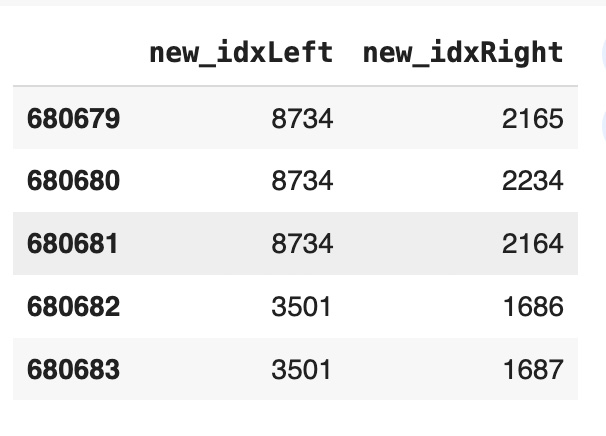
Model Training
For model training, we first used the 'all-MiniLM-L6-v2' transformer from Hugging Face to transform email texts into vectors. Next, we applied the GNN Link Prediction model from the DGL library, aiming to discover unseen graph connections by analyzing these vectors and the graph structure.- Total number of nodes: 9,654
- Total number of edges: 667,354
- Embedded nodes represented as a PyTorch tensor of size [9,654, 384]
- The output vector size for the GraphSAGE model was set to 64
Code Details
Convert edges to DGL model:unpickEdges=edges
edge_index=torch.tensor(unpickEdges[['new_idxLeft','new_idxRight']].T.values)
u,v=edge_index[0],edge_index[1]
g=dgl.graph((u,v))
g=dgl.add_self_loop(gNew)
g
Graph(num_nodes=9654, num_edges=667354,
ndata_schemes={}
edata_schemes={}) from sentence_transformers import SentenceTransformer
modelST = SentenceTransformer('all-MiniLM-L6-v2')
node_embeddings = modelST.encode(nodes['A'],convert_to_tensor=True)
node_embeddings = node_embeddings.to(torch.device('cpu'))
g.ndata['feat'] = node_embeddings
g
Graph(num_nodes=9654, num_edges=667354,
ndata_schemes={'feat': Scheme(shape=(384,), dtype=torch.float32)}
edata_schemes={}) all_logits = []
for e in range(100):
# forward
h = model(train_g, train_g.ndata['feat'].float())
pos_score = pred(train_pos_g, h)
neg_score = pred(train_neg_g, h)
loss = compute_loss(pos_score, neg_score)
# backward
optimizer.zero_grad()
loss.backward()
optimizer.step()
if e % 5 == 0:
print('In epoch {}, loss: {}'.format(e, loss)) 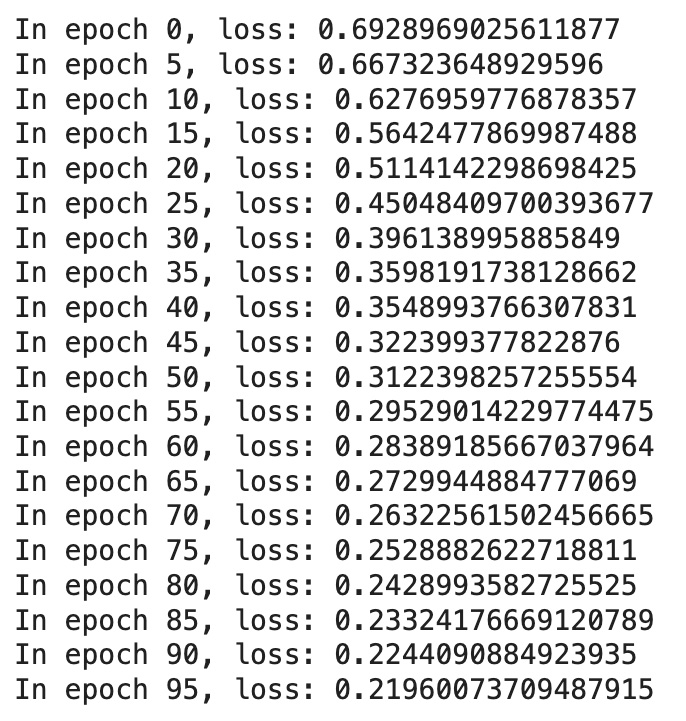
from sklearn.metrics import roc_auc_score
with torch.no_grad():
    pos_score = pred(test_pos_g, h)
    neg_score = pred(test_neg_g, h)
    print('AUC', compute_auc(pos_score, neg_score))
AUC 0.9673248461572111
Results and Further Analysis
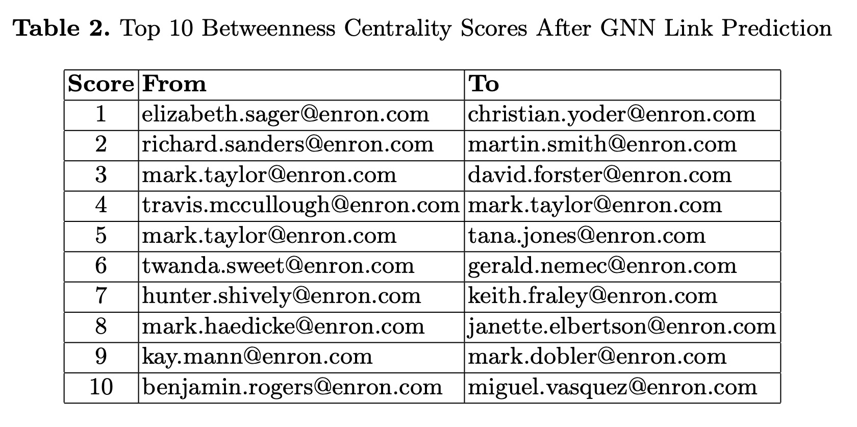
The GNN Link Prediction model outputs a set of re-embedded vectors that capture nuanced relationships within the graph. These vectors are valuable for deeper analysis, including statistical evaluation, clustering, and gaining further insights into the network’s structure. In this study, we built a new graph layer based on pairs of vectors with a cosine similarity threshold of 0.95, allowing for a detailed examination of the network’s dynamics and connections. This method enables us to observe which influencers within the network have become more or less central after introducing these new connections. For this analysis, we focused on betweenness centrality, which measures a node’s importance in a graph by indicating how often it acts as a bridge along the shortest path between two other nodes. In complex relationships, these metrics help identify key nodes that facilitate communication or interaction across the network, revealing shifts in centrality and influence based on the newly established connections.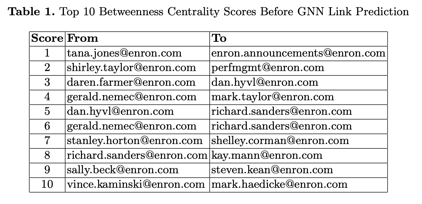 When we compare the betweenness centrality scores before and after applying our method, we observe shifts in network influence. Initially, graph connections were based solely on direct email interactions. After incorporating text-driven relationships, new dynamics and hidden connections were revealed. This significantly altered the network’s structure, uncovering previously unrecognized key connectors and providing a more comprehensive view of the network’s influence and interactions.
Code Details
Cosine Similarities function: import torch
def pytorch_cos_sim(a: Tensor, b: Tensor):
return cos_sim(a, b)
def cos_sim(a: Tensor, b: Tensor):
if not isinstance(a, torch.Tensor):
a = torch.tensor(a)
if not isinstance(b, torch.Tensor):
b = torch.tensor(b)
if len(a.shape) == 1:
a = a.unsqueeze(0)
if len(b.shape) == 1:
b = b.unsqueeze(0)
a_norm = torch.nn.functional.normalize(a, p=2, dim=1)
b_norm = torch.nn.functional.normalize(b, p=2, dim=1)
return torch.mm(a_norm, b_norm.transpose(0, 1))
cosine_scores_gnn = pytorch_cos_sim(h, h)
pairs_gnn = []
for i in range(len(cosine_scores_gnn)):
  for j in range(len(cosine_scores_gnn)):
    if i>j:
      if cosine_scores_gnn[i][j].detach().numpy() > 0.95:
        pairs_gnn.append({'idx1': i,'idx2': j,
'score': cosine_scores_gnn[i][j].detach().numpy()}) import networkx as nx
G = nx.Graph()
edges = df[df['score'] > 0.95][['idx1', 'idx2']]
edges.rename(columns={'idx1': 'source', 'idx2': 'target'}, inplace=True)
G.add_edges_from(edges.values.tolist()) betweenness_rewired = nx.betweenness_centrality(G1)
top_rewired = sorted(betweenness_rewired.items(), key=lambda x: x[1], reverse=True)[:10]